A journal of IEEE and CAA , publishes
high-quality papers in English on original
theoretical/experimental research
and development in all areas of automation
 Volume 10
Issue 6
Volume 10
Issue 6
IEEE/CAA Journal of Automatica Sinica
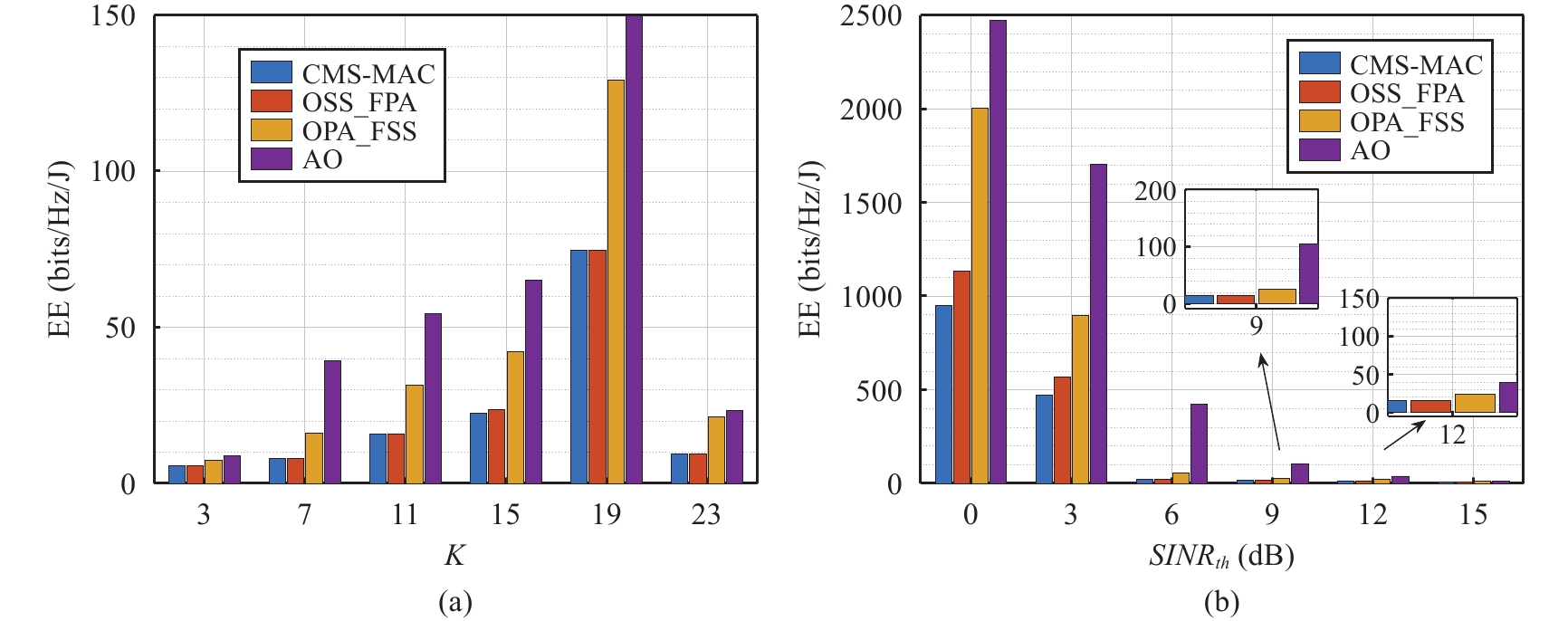
| Citation: | Z.-X. Liu, X.-C. Jin, Y.-A. Xie, and Y. Yang, “Joint slot scheduling and power allocation in clustered underwater acoustic sensor networks,” IEEE/CAA J. Autom. Sinica, vol. 10, no. 6, pp. 1501–1503, Jun. 2023. doi: 10.1109/JAS.2022.106031

|

| [1] |
L. Shi and A. O. Fapojuwo, “TDMA scheduling with optimized energy efficiency and minimum delay in clustered wireless sensor networks,” IEEE. Trans. Mob. Comput., vol. 9, no. 7, pp. 927–940, 2010. doi: 10.1109/TMC.2010.42
|
| [2] |
W. Bai, H. Wang, X. Shen, and R. Zhao, “Link scheduling method for underwater acoustic sensor networks based on correlation matrix,” IEEE Sens. J., vol. 16, no. 11, pp. 4015–4022, 2016. doi: 10.1109/JSEN.2015.2441140
|
| [3] |
M. Stojanovic, “On the relationship between capacity and distance in an underwater acoustic communication channel,” SIGMOBILE Mob. Comput. Commun. Rev., vol. 11, no. 4, pp. 34–43, 2007. doi: 10.1145/1347364.1347373
|
| [4] |
F. Xing, H. Yin, Z. Shen, and V. C. M. Leung, “Joint relay assignment and power allocation for multiuser multirelay networks over underwater wireless optical channels,” IEEE Internet Things J., vol. 7, no. 10, pp. 9688–9701, 2020. doi: 10.1109/JIOT.2020.2990925
|
| [5] |
Z. Liu, Y. Xie, Y. Yuan, K. Ma, K. Y. Chan, and X. Guan, “Robust power control for clustering-based vehicle-to-vehicle communication,” IEEE Syst. J., vol. 14, no. 2, pp. 2557–2568, 2020. doi: 10.1109/JSYST.2019.2956177
|
| [6] |
J.-P. Crouzeix and J. A. Ferland, “Algorithms for generalized fractional programming,” Mathematical Programming, vol. 52, no. 1, pp. 191–207, 1991.
|
Figures(2)


 DownLoad: