Parameters | Values |
h_1 | 0.01 |
h_2 | 1 |
h_3 | 0.1 |
γ | 8 |
δ | 8.6 |
p_1 | 20 |
p_2 | 0.1 |
α | 0.5 |
β | 1.9 |
d_1 | 1 |
d_2 | 1 |
\theta_i(0) ( i=1,\ldots,4 ) | 18 |
IEEE/CAA Journal of Automatica Sinica
Citation: | J. Y. Chai, Q. Lu, X. D. Tao, D. L. Peng, and B. T. Zhang, “Dynamic event-triggered fixed-time consensus control and its applications to magnetic map construction,” IEEE/CAA J. Autom. Sinica, vol. 10, no. 10, pp. 2000–2013, Oct. 2023. doi: 10.1109/JAS.2023.123444 |
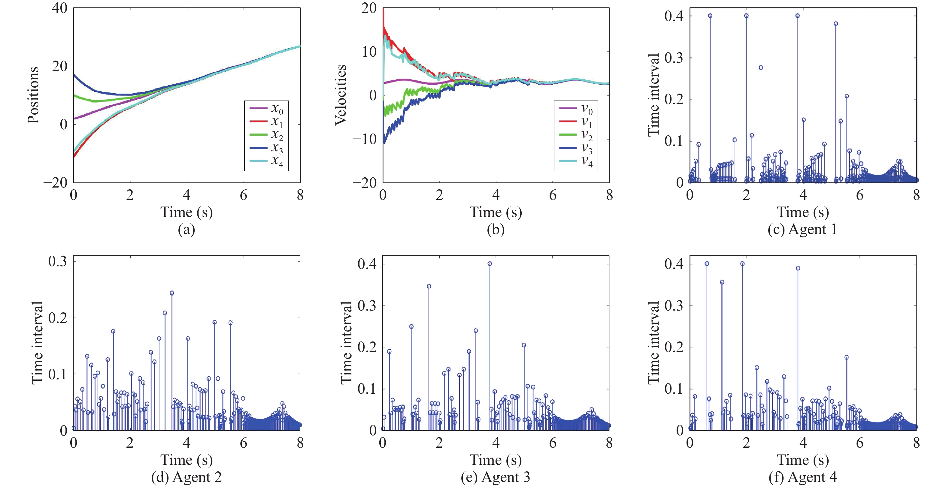
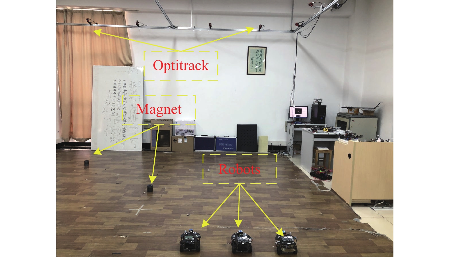
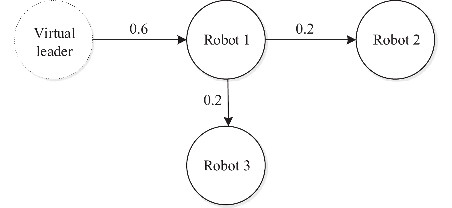
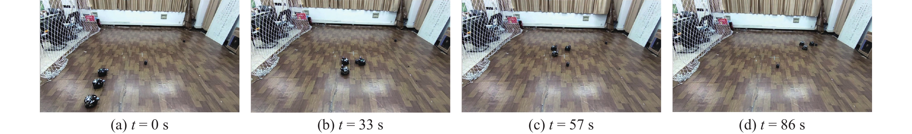
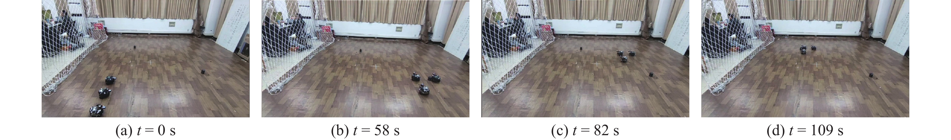
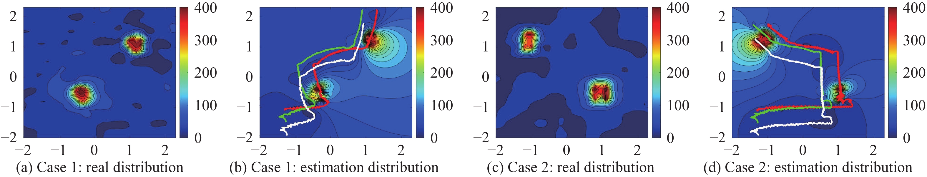
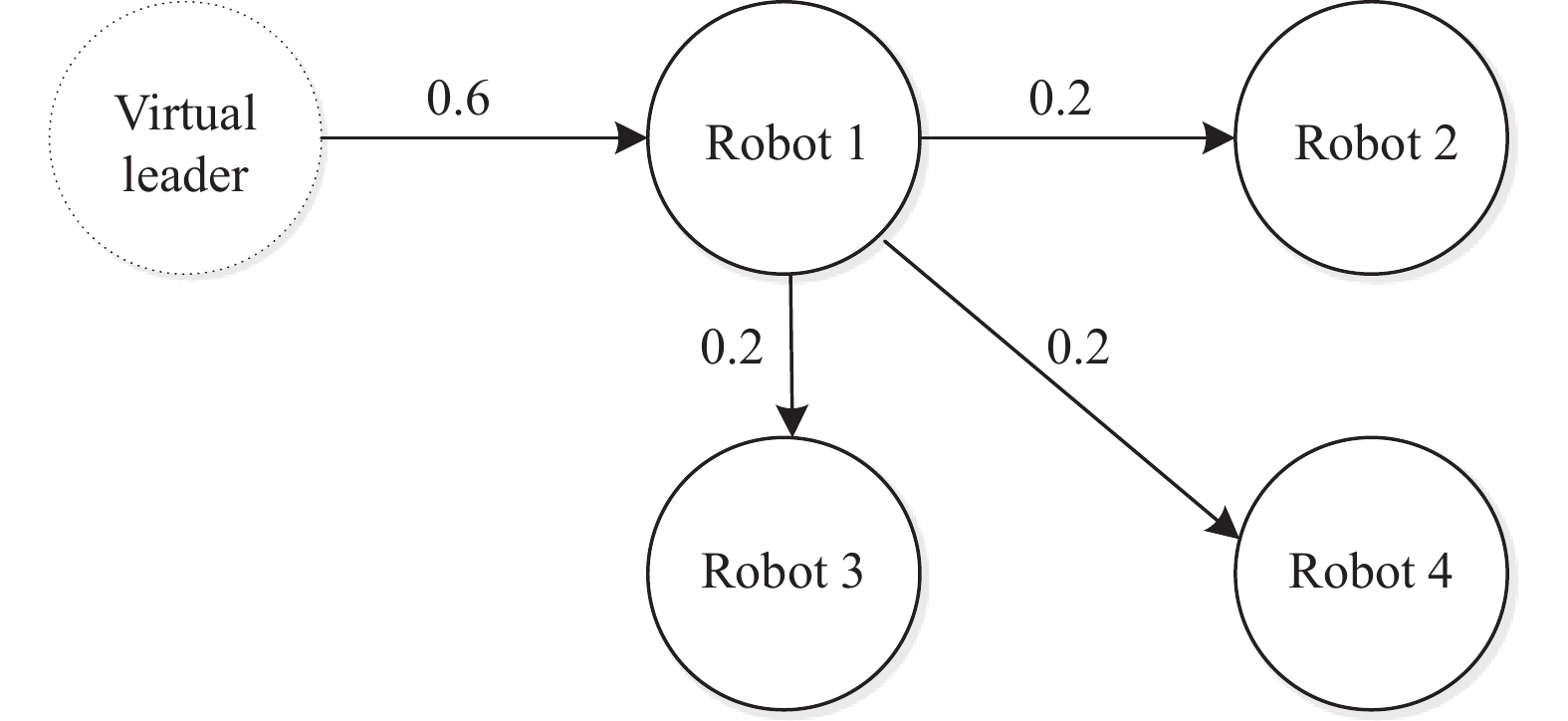
This article deals with the consensus problem of multi-agent systems by developing a fixed-time consensus control approach with a dynamic event-triggered rule. First, a new fixed-time stability condition is obtained where the less conservative settling time is given such that the theoretical settling time can well reflect the real consensus time. Second, a dynamic event-triggered rule is designed to decrease the use of chip and network resources where Zeno behaviors can be avoided after consensus is achieved, especially for finite/fixed-time consensus control approaches. Third, in terms of the developed dynamic event-triggered rule, a fixed-time consensus control approach by introducing a new item is proposed to coordinate the multi-agent system to reach consensus. The corresponding stability of the multi-agent system with the proposed control approach and dynamic event-triggered rule is analyzed based on Lyapunov theory and the fixed-time stability theorem. At last, the effectiveness of the dynamic event-triggered fixed-time consensus control approach is verified by simulations and experiments for the problem of magnetic map construction based on multiple mobile robots.
CONSENSUS control as one of the fundamental cooperative control approaches has received much attention from researchers and engineers over the last decade and has been widely applied in the fields of environmental protection and services [1]–[6]. For example, in [1], a multi-robot system based on cooperative control approaches was utilized to perform environmental perception tasks, i.e., producing electromagnetic field maps in an outdoor environment. In [4], mobile robots in terms of event-based fixed-time consensus control approaches visited positions with magnetic anomalies in a way such that the strength distribution map of magnetic fields could be accurately estimated. From the aforementioned cases, one can see that magnetic map construction is one of the main research topics in the fields of environmental protection and services because magnetic strength maps can be used to estimate soil quality degradation, to predict earthquakes from 2 weeks to a month in advance, to locate the mobile targets in the indoor environments, etc. [2], [7]–[10].
Due to several better characteristics, such as higher control accuracy, better interference suppression, and robustness to uncertainty, finite-time consensus control approaches have well studied [5], [11], [12]. But, for finite-time consensus methods, the estimated consensus time is related to the initial states of multi-agent systems. To address this case, fixed-time consensus control methods are designed where consensus time is independent with the initial states [13]–[16]. It should be pointed out that real-time controller updating and communications among agents are still required. In order to effectively reduce the use of chip and network resources, the event-triggered mechanism [17], [18] is introduced into the fixed-time consensus control approaches. It should noted that the event-triggered mechanism can only work before consensus is achieved. After consensus is achieved, Zeno behaviors cannot be avoided [19], [20]. Therefore, some researchers generally assume that the event-triggered rule can be canceled [4] in an ideal working environment after consensus is achieved. However, this kind of assumption is not real in a dynamic environment. In order to cope with this case, the dynamic event-triggered rule [17], [18], [21]–[23] is developed to avoid Zeno behavior after consensus is achieved. Due to the addition of internal variables that can be changed correspondingly with system states, the performance of the event-triggered rule is significantly improved after consensus is achieved. Notice that the dynamic event-triggered rules have been widely applied in multi-agent systems[17], [18], [22]–[24]. However, there are few researchers that have studied corresponding fixed-time consensus approaches with a dynamic event-triggered rule to coordinate the second-order nonlinear multi-agent systems.
It should be pointed out that the dynamic event-triggered fixed-time control approach for second-order nonlinear multi-agent systems not only should estimate fixed consensus time with less conservatism, but also can efficiently control multi-agent systems to save resources and avoid Zeno behaviors. However, there are two difficulties in designing the control approach for second-order nonlinear multi-agent systems under directed communication topology. One difficulty is determining how to derive a new fixed-time stability condition with less conservative settling time, which implies that the derivative item of the chosen Lyapunov functions needs to satisfy a more strict condition compared with other fixed-time stability conditions. The other difficulty is determining how to design a dynamic event-triggered rule and a fixed-time consensus approach to meet the designed fixed-time stability condition well, which means that the structure forms of the triggering rule and consensus control method need to be significantly improved. Therefore, determining how to design a fixed-time stability condition and develop a dynamic event-triggered fixed-time consensus approach to solve the aforementioned problems motivates the present studies.
This paper develops a dynamic event-triggered fixed-time consensus control approach for a second-order nonlinear multi-agent system where the proposed approach is used to cope with magnetic map construction. The main contributions are summarized in the following.
1) A new fixed-time stability condition is derived such that a less conservative settling time is obtained. The obtained condition is strict and simulation results show that the theoretical settling time obtained in this paper can reflect real consensus time well. Hence, the proposed stability condition extends and enriches the original fixed-time stability theory.
2) A dynamic event-triggered rule is designed to reduce the use of chip and communication resources by introducing an internal variable where Zeno behaviors can be avoided after consensus is achieved for finite/fixed-time consensus control approaches. Based on the proposed dynamic event-triggered rule, a fixed-time consensus control approach is developed by introducing a new item such that the proposed controller can quickly enable the second-order nonlinear multi-agent system to reach consensus.
3) The dynamic event-triggered fixed-time control approach is validated by simulation results, where one can see that the proposed control approach can control multi-agent systems to arrive at consensus with less convergence time and save chip and network resources. Then, the proposed control approach is developed to handle the problem of magnetic map construction. The experimental results demonstrate that the magnetic map can be efficiently and quickly constructed by using the proposed control approach.
The rest of this paper is organized in the following. Section II describes the dynamics model of agents. Section III presents the main contributions, that is, a new fixed-time stability condition and dynamic event-triggered fixed-time consensus control approach. Sections IV and V shows the effectiveness of the proposed approach through simulations and experiments, respectively. Finally, the conclusions are given in Section VI.
The dynamics model of the ith (i=1,…,n) agent is presented by
{˙xi(t)=vi(t)˙vi(t)=Di(xi(t),vi(t),t)+ui(t) | (1) |
where Di(xi(t),vi(t),t) is an uncertain nonlinear item; xi(t)∈Rm, vi(t)∈Rm and ui(t)∈Rm (i=1,…,n) respectively denote the ith agent’s position, velocity, and control input.
The dynamics model of a virtual leader is defined by
{˙x0(t)=v0(t)˙v0(t)=D0(x0(t),v0(t),t) | (2) |
where D0(x0(t),v0(t),t) is an uncertain nonlinear item; x0(t)∈Rm and v0(t)∈Rm are the virtual leader’s position and velocity, respectively. For the uncertain nonlinear items, we have the following assumption.
Assumption 1: Assume that the inequality ‖Di(xi(t),vi(t),t)−D0(x0(t),v0(t),t)‖≤d1‖xi(t)−x0(t)‖+d2‖vi(t)−v0(t)‖ holds where d1>0 and d2>0.
For a group of n agents, the communication among agents is modeled by a directed graph Gn(V,E,A) where V={v1,v2,…,vn} is a set of nodes, E⊂V×V is a set of edges, and A=[aij]n×n is an adjacency matrix. If the ith agent can receive the information from the jth agent, aij>0; otherwise aij=0 (i,j=1,2,…,n). Gn+1 denotes an extended graph with a virtual leader as a root node. Similarly, if the ith agent is able to receive the information from the virtual leader, ai0>0; otherwise ai0=0. Let LGn denote the Laplacian matrix of the directed graph Gn(V,E,A). Let M=LGn+diag{a10,…,an0} where diag{a10,…,an0} is a diagonal matrix with the elements a10,…,an0. And Δ=M⊗Im where the symbol ⊗ denotes Kronecker product and Im is an m-order unit matrix.
This section presents the new dynamic event-triggered fixed-time consensus control approach.
The event-triggered time sequence for the ith agent is given by
tis+1=inf | (3) |
with
\Psi_i(t)= \| \gamma e_{xi}(t)+ \delta e_{vi}(t )\| - h_1\| \gamma y_i(t_{s}^{i})+ \delta {\textit{z}}_i(t_{s}^{i})\|-h_2\theta_i(t) | (4) |
where \gamma>0 , \delta>0 , h_1>0 , h_2>0 ; t_s^i(s\in\mathbb{N},i=1,\ldots,n) is the sth time index of agent i; e_{xi}(t)=x_i(t_{s}^{i})-x_i(t) is the position error of agent i at time t; e_{vi}(t)=v_i(t_{s}^{i})-v_i(t) is the velocity error of agent i at time t; y_i(t_{s}^{i})=\sum_{j=0}^{n} a_{ij}(x_j(t_{s^\prime}^{j})-x_i(t_{s}^{i})) is the error sum of positions; {\textit{z}}_i(t_{s}^{i})=\sum_{j=0}^{n} a_{ij}(v_j(t_{s^\prime}^{j})-v_i(t_{s}^{i})) (s^{\prime}\in\mathbb{N}, j=1,\ldots,n) is the error sum of velocities; x_i(t_s^i) and x_j(t_{s^\prime}^j) are the positions of the ith agent and the jth agent at time t_s^i and time t_{s^\prime}^{j} , respectively; v_i(t_s^i) is the velocity of the ith agent at time t_s^i ; v_j(t_{s^\prime}^j) is the velocity of the jth agent at time t_{s^\prime}^{j} ; \theta_i(t) is an internal dynamical variable, which satisfies
\dot{\theta}_i(t)=-\| \gamma e_{xi}(t)+ \delta e_{vi}(t )\| +h_1\| \gamma y_i(t_{s}^{i}) + \delta {\textit{z}}_i(t_{s}^{i})\|-h_3\theta_i(t) | (5) |
where h_3>0 and \theta_i(0)>0 . Note that, based on the proposed event-triggered communication scheme (3) with (4) and (5), one obtains \dot{\theta}_i(t)\ge-(h_2+h_3)\theta_i(t) , which indicates that \theta_i(t)\ge e^{-(h_2+h_3)t}\theta_i(0) , t\ge0 . With the initial condition \theta_i(0)>0 , we have \theta_i(t)\ge 0 .
The proposed event-triggered rule requires the continuous-time position x_i(t) and velocity v_i(t) to calculate the position error e_{xi}(t) and velocity error e_{vi}(t) . When the position error e_{xi}(t) and velocity error e_{vi}(t) accumulates and reaches a certain value, the event is triggered and control input is updated; otherwise the control input holds. On the other hand, the certain value is composed of the position x_j(t_{s’}^j) and velocity v_j(t_{s’}^j) at event-triggering time, which means that the agents do not need to continuously communicate with each other. Hence, the rule is also event-triggered communication rule, which can save network resources. Moreover, the continuous-time position x_i(t) and velocity v_i(t) can be obtained by the corresponding sensors. The control input is only calculated at the event-triggering time, which implies that chip resources are saved.
Remark 1: It should be pointed out that, after consensus is achieved, e_{vi}(t)=0 , y_i(t_s^i)=0 and {\textit{z}}_i(t_s^i)=0 . Due to e_{xi}(t)\neq 0 , the condition (3) is satisfied in the static event-triggered condition, which results in Zeno behaviors. By introducing the variable \theta_i(t) , the variable \theta_i(t)>0 after consensus can avoid Zeno behaviors. Hence, \theta_i(t) presented by (5) is important to avoid Zeno behaviors.
Remark 2: The proposed dynamic event-triggered communication rule (3) with (4) and (5) has two advantages compared with our previous results in [4]. One advantage is that our previous results [4] show that Zeno behaviors can occur after consensus is achieved if the multi-agent system still needs to communicate with each other while Zeno behaviors do not occur after consensus is achieved for the proposed scheme. The other advantage is that, due to using the internal variable \theta_i(t) , the performance capabilities of event triggering for the proposed scheme is better than the ones for our previous approaches [4]. Moreover, when h_2=0 , the proposed approach degrades the previous approaches [4]. Hence, our previous approaches [4] can be considered as a particular case of the proposed approach. However, the proposed event-triggered rule has several limitations. Compared with the other event-triggered rule [4], we need to set more parameters, which are important for event-triggering results. Moreover, due to introducing the variable \theta_i , the proposed-event-triggered rule is more complicated, which increases the computational complexity.
Remark 3: The dynamic event-triggered rules have been widely used in multi-agent systems [17], [18], [24]. However, it is noteworthy that there are two different characteristics between the proposed dynamic event-triggered rule and the current dynamic event-triggered rules in [17]–[19], [22]–[24]. The first characteristic is that the proposed dynamic event-triggered rule is designed for the second-order nonlinear multi-agent system with fixed-time consensus control while the other dynamic event-triggered rules are developed for the multi-agent system with general consensus control. The second characteristic is that the proposed dynamic event-triggered approach can reduce the use of the chip and communication resources of multi-robot systems whereas some approaches in [17]–[19], [24] only save chip resources and still need the real-time information exchange.
On the basis of the aforementioned dynamic event-triggered rule (3) with (4) and (5), inspired by [25], the fixed-time consensus controller is proposed by
u_i(t)= \mathrm{sig}(\phi_i(t))^{\alpha}+\mathrm{sig}(\phi_i(t))^{\beta}+\Bigg(p_1 + \frac{p_2}{\|\phi_i(t)\|^2}\Bigg)\phi_i(t) | (6) |
with
\begin{eqnarray} \phi_i(t)=\sum\limits_{j=0}^{n}a_{ij}(\gamma(x_j(t_{s^\prime}^j)-x_i(t_s^i)) +\delta(v_j(t_{s^\prime}^j)-v_i(t_s^i)) \end{eqnarray} | (7) |
where \mathrm{sig}\;(\phi_i(t))^\alpha\;=\;[\mathrm{sign}\;(\phi_{i1})|\phi_{i1}|^\alpha,\;\ldots,\;\mathrm{sign}\;(\phi_{im})|\phi_{im}|^\alpha]^T; \mathrm{sig}(\phi_i(t))^\beta\;=\;[\mathrm{sign}(\phi_{i1})|\phi_{i1}|^\beta,\ldots,\mathrm{sign}(\phi_{im})|\phi_{im}|^\beta]^T; 0<\alpha<1 ; \beta>1 ; p_1>0 , p_2>0 ; m is the dimensions of positions and velocities. Moreover, we define that {\phi_i(t)}/{\|\phi_i(t)\|^2}=0 when \phi_i(t)=0 .
Remark 4: Compared with our previous fixed-time consensus approaches [4], [19], the proposed approach has one important characteristic, which is that the item {\phi_i(t)}/{\|\phi_i(t)\|^2} is introduced into (6). As a result, the estimated settling time more accurately reflects the real convergence time compared to the ones in [4], [19]. Hence, the estimated settling time has good guidance for parameter design and task execution. Moreover, different from the other fixed-time consensus approaches [19], [20], [26], the proposed approach can control the agents with second-order nonlinear dynamics while the other fixed-time consensus approaches [19], [20], [26] only can coordinate agents with the first-order linear kinematics. Hence, the other fixed-time consensus approaches [19], [20], [26] can be viewed as the particular cases of the proposed approach.
Before giving the consensus theorem, the following globally fixed-time stability condition is shown as:
Theorem 1: Suppose that V:\mathbb{R}^n \to \mathbb{R}_+ \bigcup 0 is a continuous radially unbounded function and satisfies: 1) V(x_t)=0 when x_t=0 ; 2) Inequality \dot{V}(x_t) \leq -aV(x_t) -bV^{\hat{\alpha}}(x_t)- cV^{\hat{\beta}}(x_t)- d for any solution x_t where a, b,c,d>0 , 0<\hat{\alpha}<1 , \hat{\beta}>1 . Therefore, the system \dot{x}_t=f(x_t) is globally fixed-time stable and the settling time T_0 satisfies
\begin{equation*} T_0 \leq \frac{1}{\sqrt{bd}(2-\hat{\alpha})}\Bigg(\sqrt{\frac{bd}{ac}}\Bigg)^\frac{2-\hat{\alpha}}{\hat{\beta}+1-\hat{\alpha}} +\frac{1}{\sqrt{ac}(\hat{\beta}-1)}\Bigg(\sqrt{\frac{bd}{ac}}\Bigg)^\frac{1-\hat{\beta}}{\hat{\beta}+1-\hat{\alpha}}. \end{equation*} |
Proof: See the Appendix A.
Remark 5: From Theorem 1, one can see that the given condition \dot{V}(x_t) \leq -aV(x_t) -bV^{\hat{\alpha}}(x_t)-cV^{\hat{\beta}}(x_t)-d provides a more strict result compared with the references [4], [27], [28] such that the settling time T_0 derived in Theorem 1 is less conservative than the one obtained in [4], [27], [28]. This paper provides the possibility to predefine the system parameters according to the fixed communication topology. However, the parameter d is hard to be given, which requires that we should carefully design the dynamic event-triggered fixed-time controller.
By using the proposed dynamic event-triggered fixed-time consensus control (6), the following theorems are given to ensure that consensus is obtained within a fixed-time interval.
Theorem 2: Assume a fixed directed communication topology G_{n+1} with a spanning tree. The virtual leader is a root node in the spanning tree. For the multi-agents system with the proposed control approach (6) under the dynamic event-triggered rule (3) with (4) and (5), if \delta > \max\{\sqrt{\gamma/ ( p_1\mu_{\min}}), {d_2}/{\sqrt{\theta_{\min}(\Delta^T\Delta)}}\}, \gamma \geq {d_1}/{\sqrt{\theta_{\min}(\Delta^T\Delta)}}, and
\begin{align*} h_1<&\min \Bigg\{ \frac{1}{\|\Delta\|(1+h_2b_t)}, \frac{k_1}{(1+h_2b_t)\|\Delta\|^2(nm)^{\frac{\beta-1}{2}}}, \\ & \frac{k_2}{(1+h_2b_t)\|\Delta\|^2(nm)^{\frac{1-\alpha}{2}}}, \frac{\frac{1}{2}\mu_{\min}}{(1+h_2b_t)\|\Delta\|^2},\\ &\frac{\frac{1}{2}p_1\gamma^2\mu_{\min}-2\gamma^2\|\Delta\|}{\|\Delta\|(1+h_2b_t)(p_1\gamma^2\|\Delta\|+\frac{1}{2}p_1\gamma^2\mu_{\min}-2\gamma^2\|\Delta\|)},\\ &\frac{\frac{1}{2}p_1\delta^2\mu_{\min}-\gamma-2\delta^2\|\Delta\|}{\|\Delta\|(1+h_2b_t)(p_1\delta^2\|\Delta\|+\frac{1}{2}p_1\delta^2\mu_{\min}-\gamma-2\delta^2\|\Delta\|)}\Bigg\} \end{align*} |
then, within a fixed-time interval, the multi-agent system reaches consensus.
The estimated settling time T_0 is given by
\begin{equation*} T_0 \leq \frac{2}{\sqrt{bd}(3-\alpha)}\Bigg(\sqrt{\frac{bd}{ac}}\Bigg)^\frac{3-\alpha}{\beta+2-\alpha}+\frac{2}{\sqrt{ac}(\beta-1)}\Bigg(\sqrt{\frac{bd}{ac}}\Bigg)^\frac{1-\beta}{\beta+2-\alpha} \end{equation*} |
with
\begin{align*} &a=\frac{2}{\lambda_{\max}} \min\Bigg\{\frac{1}{2}p_1\gamma^2\mu_{\min}-\frac{p_1\gamma^2\|\Delta\|^2 (h_1+h_2h_1b_t)}{ 1-\parallel\Delta\parallel(h_1+h_2h_1b_t)}\\&\qquad-2\gamma^2\|\Delta\|,\\&\qquad\frac{1}{2}p_1\delta^2\mu_{\min}-\frac{p_1\delta^2\|\Delta\|^2 (h_1+h_2h_1b_t)}{ 1-\parallel\Delta\parallel(h_1+h_2h_1b_t)} -\gamma-2\delta^2\|\Delta\|\Bigg\}\\ &b=\frac{k_1-(h_1+h_2h_1b_t)\|\Delta\|^2(nm)^{\frac{1-\alpha}{2}}}{(\frac{\lambda_{\max}}{2\jmath \min\{\gamma^2,\delta^2\}})^{\frac{1+\alpha}{2}}}\\ &c=\frac{k_2-(h_1+h_2h_1b_t)\|\Delta\|^2(nm)^{\frac{\beta-1}{2}}}{(\frac{\lambda_{\max}}{2\jmath \min\{\gamma^2,\delta^2\}})^{\frac{1+\beta}{2}}(nm)^{\frac{\beta-1}{2}}}\\ &d=p_2(\frac{1}{2}\mu_{\min}-\|\Delta\|^2h_1(1+h_2b_t)) \end{align*} |
where b_t is the upper bound of all the neighboring event intervals; k_1=\min_{i=1,\ldots,n}\{\frac{\alpha}{\alpha+1}(\sum_{j=1}^{n}a_{ij} - \sum_{j=1}^{n}a_{ji})+a_{i0}\} ; k_2= \min_{i=1,\ldots,n}\{\frac{\beta}{\beta+1}(\sum_{j=1}^{n}a_{ij} - \sum_{j=1}^{n}a_{ji})+a_{i0}\} ; \lambda_{\max} is the maximal eigenvalue of the matrix Π in Appendix B; \mu_{\min} is the minimal eigenvalue of the matrix \Delta+\Delta^T ; \theta_{\min} is the minimal eigenvalue of the matrix \Delta^T\Delta .
Proof: See Appendix B.
Remark 6: From Theorem 2, one can see that, compared with the other theorems involving multi-agent systems with the fixed-time consensus approach [19], [20], [26], the use of Theorem 1 significantly reduces the conservatism of the settling time T_0 such that Theorem 2 can accurately estimate consensus time of multi-agent systems with the proposed control approach (6) under the dynamic event-triggered scheme (3) with (4) and (5).
The following corollary is directly given for multi-agent systems with a fixed undirected communication topology.
Corollary 1: Assume a fixed undirected communication \mathcal{G}_{n+1} with a spanning tree. The virtual leader is a root node in the spanning tree. For a multi-agent system with the proposed control approach (6) under dynamic event-triggered rule (3) with (4) and (5), if {\delta} > \max\{\sqrt{{\gamma}\nu_{\max}/ {p}_1}, {d_2}/{\sqrt{\theta_{\min}(\Delta^T\Delta)}}\} ( \nu_{\max} is the maximal eigenvalue of \Delta^{-1} ), {\gamma} \geq {d_1}/{\sqrt{\theta_{\min}(\Delta^T\Delta)}}, and
\begin{align*} {h}_1<&\min \Bigg\{ \frac{1}{(1+h_2b_t)\|\Delta\|(nm)^{\frac{\beta-1}{2}}}, \\ & \frac{1}{(1+h_2b_t)\|\Delta\|(nm)^{\frac{1-\alpha}{2}}},\\ &\frac{p_1{\delta}^2-{\gamma} \nu_{max} -2{\delta}^2}{\|\Delta\|(1+h_2b_t)(2 p_1{\delta}^2 -{\gamma} \nu_{max}-2{\delta}^2)}\Bigg\} \end{align*} |
then the multi-robot system reaches consensus within a fixed-time interval and there are no Zeno behaviors.
The estimated settling time \hat{T}_0 is given by
\begin{equation*} {T}_0 \leq \frac{2}{\sqrt{{b}{d}}(3-\alpha)}\Bigg(\sqrt{\frac{{b}{d}}{{a}{c}}}\Bigg)^\frac{3-\alpha}{\beta+2-\alpha}+\frac{2}{\sqrt{{a}{c}}(\beta-1)}\Bigg(\sqrt{\frac{{b}{d}}{{a}{c}}}\Bigg)^\frac{1-\beta}{\beta+2-\alpha} \end{equation*} |
with
\begin{align*} &{a}=\frac{2}{{\lambda}_{\max}} \min\Bigg\{p_1{\gamma}^2-2{\gamma}^2- \frac{p_1{\gamma}^2\|\Delta\| ({h}_1+h_2{h}_1b_t)}{ 1-\parallel\Delta\parallel({h}_1+h_2{h}_1b_t)},\\ &\qquad p_1{\delta}^2-{\gamma}\nu_{\max}-2{\delta}^2-\frac{p_1{\delta}^2\|\Delta\| ({h}_1+h_2{h}_1b_t)}{ 1-\parallel\Delta\parallel({h}_1+h_2{h}_1b_t)}\Bigg\}\\ &{b}=\frac{1-({h}_1+h_2{h}_1b_t)\|\Delta\|(nm)^{\frac{1-\alpha}{2}}}{(\frac{{\lambda}_{\max}}{\jmath \min\{{\gamma}^2,{\delta}^2\}})^{\frac{1+\alpha}{2}}}\\ &{c}=\frac{1-({h}_1+h_2{h}_1b_t)\|\Delta\|(nm)^{\frac{\beta-1}{2}}}{(\frac{{\lambda}_{\max}}{\jmath \min\{{\gamma}^2,{\delta}^2\}})^{\frac{1+\beta}{2}}(nm)^{\frac{\beta-1}{2}}}\\ &{d}=p_2(1-\|\Delta\|\hat{h}_1(1+h_2b_t)). \end{align*} |
In what follows, we give Theorem 3 to illustrate that there are no Zeno behaviors for the multi-agent system with the proposed control approach and the dynamic event-triggered rule.
Theorem 3: For the multi-agent system (1), Zeno behaviors do not occur due to have a minimum inter-execution interval \tau^*>0 when using the proposed dynamic event-triggered rule (3) with (4) and (5).
Proof: See Appendix C.
Remark 7: From Theorem 3, one can see that there exists a minimum inter-execution interval which is a strictly positive constant \tau^* . Moreover, because we introduce the dynamical variable \theta_i(t) , after consensus is arrived, Zeno behaviors do not appear. But, it is worth mentioning that Zeno behaviors can occur for the other event-triggered schemes [19], [20] after consensus is obtained. Hence, the proposed event-triggered rule can efficiently deal with Zeno behaviors.
The proposed dynamic event-triggered fixed-time consensus (DEFC) control approach is summarized in Algorithm 1.
Algorithm 1 The DEFC control approach
Input: γ, δ, h_1 , h_2 , h_3 , \theta_i(0) , α, β, p_1 , p_2 , x_i(0) , and v_i(0) , i=1,\ldots,n
Output: u_i(t) , i=1, \ldots, n
1 while: i\leq n do
2 if The neighbors’ positions and velocities are obtained then
3 Save the neighbors’ triggering time, positions, and velocities as the new information;
4 else
5 Use the neighbors’ positions and velocities at the last event-triggering time;
6 end
7 Compute the dynamic event-triggered condition in terms of (3) with (4) and (5);
8 if \Psi_i(t)\leq0 then
9 The event-triggering time is unchanged;
10 else
11 The event-triggering time is updated;
12 Transmit v_i(t_s^i) and x_i(t_s^i) into its neighbors when the event is triggered;
13 end
14 Compute the u_i(t) in (6) for the ith robot in the light of the saved event-triggering time;
15 end
Remark 8: In Algorithm 1, the choice of parameters is significant. The parameters d_1 and d_2 depend on the nonlinear item. For different nonlinear items, the parameters d_1 and d_2 are different. The parameters α and β have little impact on convergence velocity. Hence, the two parameters are set according to constraints. Moreover, increasing \theta_i(0) can generate good event-triggering results. But, the convergence velocity is slow. Thus, the parameter \theta_i(0) is set as an appropriate value. The parameters h_1 , h_2 , and h_3 have an influence on event-triggering performance. However, if the parameters are big value, system stability is influenced by Theorem 2. Hence, the three parameters are set to be a small value. Finally, the parameters δ, γ, p_1 , and p_2 are set according to Theorem 2.
This section illustrates the effectiveness of the DEFC control approach (Algorithm 1).
To consider the multi-agent system (1) with four agents ( i=1,\ldots,4 ) and a virtual leader (2), where \mathcal{D}_i(x_i(t),v_i(t),t)= -\;1.5\cos(x_i(t))\; \;+\;\; \sin(v_i(t)) and \mathcal{D}_0\;(x_0(t),\;v_0(t),\;t)\;= -1.5\times \cos(x_0(t)) + \sin(v_0(t)). Under Theorem 2, the parameters of Algorithm 1 are shown in Table I. The communication topology is a fixed directed graph, as shown in Fig. 1. The initial positions and velocities of four robots are stochastically generated among [-17,17] and [-1.4,1.4] , respectively. The initial position and velocity of the virtual leader are x_0(0)=2 and v_0(0)=2.8 , respectively. Moreover, the maximal time interval of event triggering b_t is set as 0.4 s. The sampling time is 0.001 s with a total running time of 8 s.
Parameters | Values |
h_1 | 0.01 |
h_2 | 1 |
h_3 | 0.1 |
γ | 8 |
δ | 8.6 |
p_1 | 20 |
p_2 | 0.1 |
α | 0.5 |
β | 1.9 |
d_1 | 1 |
d_2 | 1 |
\theta_i(0) ( i=1,\ldots,4 ) | 18 |
In order to estimate prediction capabilities of the settling time from the proposed Theorem 1, we choose three widely used fixed-time stability conditions from [16], [27], [29]. The upper bounds of convergence time of the proposed DEFC control approach are theoretically estimated according to the different estimated approaches, and the corresponding results are shown in Table II.
On the other hand, the proposed DEFC approach is repeatedly executed over 50 runs. The real mean consensus time is 7.3933 s with the standard deviation 0.4536 s under the convergence precision 0.005. From Table II, one can see that, the obtained settling time is smaller than the one calculated by the state of the art conditions in [16], [27], [29], which means that the settling time from Theorem 1 can reflect the real consensus time well.
Moreover, when the initial positions of four robots are x_1(0)=-11 , x_2(0)=10 , x_3(0)=17 , x_4(0)=-9 , and the initial velocities of four robots are v_1(0)=1.4 , v_2(0)=0.5 , v_3(0)= -1.2 , v_4(0)=-0.1 , consensus is arrived at t= 7.998 s. When t=10 s, we can achieve \theta_1(t)=0.02 , \theta_2(t)=0.05 , \theta_3(t)=0.07 , and \theta_4(t)=0.04 , which implies that Zeno behaviors do not occur after consensus is arrived.
Table III shows the event-triggered ratio, which can be computed by division between the updating number and total number. Notice that the recent event-triggered fixed-time consensus control approaches [19], [20] are mainly employed for first-order multi-agent systems and are not appropriate for handling the second-order nonlinear multi-agent systems. Hence, the comparison approach is selected from [4] where the second-order nonlinear multi-agent system is considered. From Table III, one can see that the event-triggered ratio obtained by the DEFC approach is much better than the one received in [4] under the same conditions. The parameters in [4] have been carefully adjusted. However, the event-triggered results are not good. The main reason is that the Zeno behaviors occur after consensus is achieved.
Methods | Agent 1 | Agent 2 | Agent 3 | Agent 4 |
DEFC | 4.06 (0.40) | 2.68 (0.25) | 2.61 (0.31) | 2.62 (0.28) |
Lu et al. [4] | 13.63 (10.92) | 16.17 (12.91) | 14.40 (12.71) | 20.04 (19.84) |
Figs. 2(a) and 2(b) show the convergence processes of positions and velocities for four agents in a run. Figs. 2(c)−2(f) illustrate the corresponding time interval of four agents. From Fig. 2, one can see that the convergence velocity can be improved because of the introduction of the item {\phi_i(t)}/{\|\phi_i(t)\|^2} in (6). It should be pointed out that, if the convergence velocity is accelerated, then the event-triggered results become poor. Otherwise, if the event-triggered results are good, then the convergence velocity becomes slow. Hence, this is a trade-off problem, which can dealt with according to the real application requirements.
This section uses the proposed DEFC approach to control a multi-robot system to construct magnetic maps in an indoor environment. It is worth mentioning that the leader-follower structure is employed for multi-robot systems where the magnetic anomaly positions are regarded as a virtual leader such that the followers can reach magnetic anomaly positions within a fixed-time interval.
Fig. 3 shows the experimental environment 4 m \times 4 m. It is worthwhile to indicate that three robots are employed to construct the strength distribution map of magnetic fields where two magnets are placed to simulate the magnetic anomaly area [30]. Each magnet is a hexagonal cylinder with outer diameter of 80 mm and inner diameter of 38 mm. In order to show the effectiveness of the DEFC approach, two cases with different magnetic anomaly positions, denoted by Cases 1 and 2, are considered. For Case 1, two magnets are placed in [−0.34, −0.57] and [1.12, 1.08], respectively. For Case 2, two magnets are placed in [0.94, −0.53] and [−1.08, 1.21], respectively. The main differences of two cases are that the magnets are relatively placed in the different quadrants. Magnets are placed in the first quadrant and the third quadrant for Case 1 while magnets are placed in the second quadrant and the fourth quadrant for Case 2. For each case, ten real experiments are conducted to ensure the reliability of the experimental results. Moreover, the mobile robots install the magnetic sensors RM3100. The control board is Raspberry Pi 3b+, in which ROS is run. The programming language is C++ [31].
In order to construct the magnetic map, the multi-robot system needs to keep a formation to sample magnetic information over a wide area. Hence, (7) can be further modified as
\begin{split} \phi_i(t)=\;&\sum\limits_{j=0}^{n}a_{ij}(\gamma((x_j(t_{s^\prime}^j)-d^j)-(x_i(t_s^i)-d^i))\\ &+\delta(v_j(t_{s^\prime}^j)-v_i(t_s^i)) \end{split} | (8) |
where d^1=[0,0]^T , d^2=[0.5,0]^T , d^3=[0,0.5]^T , and d^0 = 0 . In the next experiments, the proposed DEFC approach with (8) instead of (7) is used to control the multi-robot system to perform the magnetic map construction task. According to the estimated consensus time in Table II, the parameters of the DEFC approach are similar with the parameters used in the simulation section except for p_1=10 and \theta_i(0)=580 ( i= 1,\ldots,3 ). Decreasing the p_1 can improve the smoothness of velocity changing and increasing the \theta_i(0) can improve the performance of the dynamic event-triggered rule. The communication topology is shown in Fig. 4. Moreover, there are two aspects to be considered for the use of the DEFC approach. One aspect is that, if any robots detect the magnetic strength, then the virtual leader is run in this robot. The virtual leader’s position is set in terms of the Gaussian process and its velocity is zero. The other aspect is that, the sampling time is set as 0.01 s in order to match the prediction time of Gaussian process.
The above dynamics and control scheme are based on the “hand position”. According to the results from the references [4], [32], [33], the “hand position” is used to take place of “center position” of the robot. The dynamics at the “center position” of the differential robots can be described by
\left( \begin{array}{c} \dot{r}_{xi} \\ \dot{r}_{yi} \\ \dot{\varphi}_i \\ \dot{\nu}_i \\ \dot{\omega}_i \\ \end{array} \right) =\left( \begin{array}{c} \nu_i\mathrm{cos}\varphi_i \\ \nu_i\mathrm{sin}\varphi_i \\ \omega_i \\ 0 \\ 0 \\ \end{array} \right) +\left( \begin{array}{cc} 0 & 0 \\ 0 & 0 \\ 0 & 0 \\ \dfrac{1}{m_i} & 0 \\ 0 & \dfrac{1}{J_i} \\ \end{array} \right)\left( \begin{array}{c} F_i \\ \tau_i \\ \end{array} \right) | (9) |
where r_i=(r_{xi}, r_{yi})^T is the position of the i{\mathrm{th}} robot; \nu_i and \omega_i are the linear velocity and angular velocity, respectively; \tau_i and F_i the torque and force, respectively; m_i is the mass; and J_i is the moment of inertia. Let I_i=(F_i, \tau_i)^T be the control input. The relationship of control inputs between the “hand position” and the “center position” can be described by
\begin{split} I_i =\;& \left( \begin{array}{cc} \dfrac{1}{m_i}\mathrm{cos}\varphi_i & -\dfrac{L_i}{J_i}\mathrm{sin}\varphi_i \\ \dfrac{1}{m_i}\mathrm{sin}\varphi_i & \dfrac{L_i}{J_i}\mathrm{cos}\varphi_i \end{array} \right)^{-1}\\&\times\left[u_i-\left( \begin{array}{c} -\nu_i\omega_i\mathrm{sin}\varphi_i -L_i\omega_i^2\mathrm{cos}\varphi_i\\ \nu_i\omega_i\mathrm{cos}\varphi_i -L_i\omega_i^2sin\varphi_i \end{array} \right) \right] \end{split} | (10) |
where \varphi_i denotes the orientation; L_i is a distance between “hand position” and “center position” along the line that is perpendicular to the wheel axis.
We use three performance metrics to show the effectiveness of the DEFC approach for the problem of magnetic map construction. The first metric is localization error, which can be calculated by
LE_i - \frac{1}{n}\sum\limits_{j=1}^n\|\hat{s}_j-s_i\| | (11) |
where \hat{s}_j is the estimated position for the jth robot; s_i is the ith real position with magnetic anomaly; and LE_i is the localization error of the ith magnetic anomaly position. It is noted that, in order to quickly construct the magnetic map, during the traversal process, mobile robots are required to visit the magnetic anomaly position because the magnetic strength distribution in the search environment is significantly influenced by the strength at the magnetic anomaly position. Hence, localization error is an important indicator for magnetic map construction.
The second metric is the event-triggered ratio ER_i , which can be computed by division of the updating number by the total number. This metric has been widely used to estimate the performance of event-triggered schemes and can be found in some literature [4], [18], [19].
The third metric is the the map error, which can be obtained by
ME = \sqrt{\frac{1}{L}\sum\limits_{j=1}^L \Bigg(\frac{1}{n}\sum_{i=1}^n\hat{c}_{ij}-c_j\Bigg)^2} | (12) |
where L=1600 is the cell number in the search environment; \hat{c}_{ij} is the estimated magnetic strength of the ith robot at the jth cell; c_j is the real magnetic strength at the center of the jth cell; and ME is the map error. Note that ME can indicate the accuracy of magnetic map. Since the purpose of this paper is to construct a magnetic map with small map errors, mobile robots are required to cover a wide area during the traversal process.
Figs. 5 and 6 show the traversal process of three mobile robots for Cases 1 and 2, respectively. From these figures, one can see that, during the traversal process, if the mobile robots detect magnetic strength, then these robots move toward the positions with magnetic anomalies according to the decision results of the Gaussian process. After visiting the positions with magnetic anomalies, three robots continue to start the traversal process. Moreover, one can also see that the positions with magnetic anomalies can be found for Cases 1 and 2.
Figs. 7(a) and 7(b) illustrate the real magnetic distribution and the estimated magnetic distribution for Case 1, respectively. Figs. 7(c) and 7(d) illustrate the real magnetic distribution and the estimated magnetic distribution for Case 2, respectively. From Fig. 7, one can see that, under the control of the proposed DEFC approach, mobile robots can find the positions with magnetic anomalies and quickly keep a formation when the virtual leader changes its position. The estimated magnetic distribution reflects the real magnetic distribution well. Note that the magnetic anomalies influence a certain area and magnetic strength in other areas are uniform distribution. If the magnetic strength more than the threshold (50 uT) is detected, a Gaussian process is used to predict a position for the virtual leader. Mobile robots change their behaviors going from the traversal process to localization process. From Figs. 7 (b) and 7(d), it is observed that the proposed DEFC approach enables the robots to keep a formation quickly during the switching process.
Table IV describes the localization errors for two cases, from which one can see that the average localization error is small over 10 runs. However, the instability of magnetic sensors leads to the prediction difficulty of anomaly positions for several experiments and several big localization errors are obtained. Table V gives the event-triggered ratio, from which one can also see that the proposed DEFC approach can save the chip and communication resources. Compared with the simulation results, the event-triggered ratio becomes bigger. One main reason is that, after visiting the positions with magnetic anomalies, the mobile robots conduct the traversal process. Since the proposed DEFC approach can control the mobiles robots to quickly keep a formation during the traversal process, the dynamic variable \theta_i(t) in (5) has a significant impact on the triggering ratio. Although the use of the dynamic variable \theta_i(t) can avoid the appearance of Zeno behaviors after consensus is achieved, the triggering ratio still increases due to the decrease of \theta_i(t) . Table VI shows the map errors. From this table, one can see that the map error is small and the estimated magnetic map can reflect the real magnetic map well.
Case | Source | Max | Min | Mean | Std |
Case 1 | Source 1 | 0.10 | 0.01 | 0.07 | 0.04 |
Source 2 | 0.17 | 2.6×10⁻⁴ | 0.07 | 0.08 | |
Case 2 | Source 1 | 0.14 | 0.06 | 0.10 | 0.02 |
Source 2 | 0.14 | 6.2×10⁻⁴ | 0.11 | 0.04 |
Case | Index | Robot 1 | Robot 2 | Robot 3 |
Case 1 | Max | 22.79 | 17.05 | 16.02 |
Min | 14.33 | 9.24 | 9.81 | |
Mean | 17.56 | 11.88 | 12.19 | |
Std | 2.68 | 2.84 | 2.10 | |
Case 2 | Max | 20.31 | 15.58 | 15.51 |
Min | 17.05 | 12.04 | 12.39 | |
Mean | 18.87 | 13.40 | 13.65 | |
Std | 1.15 | 1.07 | 0.93 |
Case | Max | Min | Mean | Std |
Case 1 | 52.57 | 32.45 | 44.76 | 6.24 |
Case 2 | 51.90 | 31.66 | 40.90 | 7.06 |
On the basis of the multi-agent system, the consensus problem has been addressed. First, we have given a new and less conservative fixed-time stability condition in order to enable the theoretical prediction time to well reflect the real consensus time. Then, we have designed a dynamic event-triggered communication rule to cope with the problem of Zeno behaviors for finite/fixed-time consensus control approaches after consensus is arrived. Next, we have proposed a fixed-time consensus control approach based on the dynamic event-triggered communication rule. Finally, we illustrate the effectiveness of the proposed DEFC approach for magnetic map construction by using multiple mobile robots.
In future, we will consider fixed-time consensus algorithms with different forms, which can satisfy the different dynamics requirements and Theorem 1. We will also consider dynamic event-triggered rules without position items in order to obtain good event-triggering performance. Moreover, for the problem of magnetic map construction, we will study the data processing approach to predict the positions of magnetic sources in order to quickly arrive at the positions and accurately plot the magnetic map. We will also co-design the reinforcement learning and dynamic event-triggered fixed-time consensus approach such that decision and control forms a closed loop.
Proof: Since \dot{V}(x_t) \leq -aV(x_t) -bV^{\hat{\alpha}}(x_t)-cV^{\hat{\beta}}(x_t)-d and x_0\neq 0 is the initial state, it is straightforward to obtain
\dot{V}(x_t) \leq -d . | (13) |
By solving (13), we get T_0={V(x_0)}/{d}>0 , which implies that \lim_{t\rightarrow T_0} V(x_t)= 0 and V(x_t)=0 when t>T_0 . Hence, the starting position of the system \dot{x}_t=f(x_t) is a globally fixed-time stable equilibrium.
By taking similar steps in [28], [34], we have
\begin{split} T_0=\;& \int_0^{T_0} {dt}\leq \int_{V(x_0)}^0 \frac{1}{-as -bs^{\hat{\alpha}}-cs^{\hat{\beta}}-d} {ds}\\ =\;&\int^{r}_0 \frac{1}{as +bs^{\hat{\alpha}}+cs^{\hat{\beta}}+d}{ds}\\&+\int^{V(x_0)}_r \frac{1}{as +bs^{\hat{\alpha}}+cs^{\hat{\beta}}+d}{ds}\\ \leq \;&\int^{r}_0 \frac{1}{2\sqrt{bd}s^{\frac{{\hat{\alpha}}}{2}}}{ds}+\int^{V(x_0)}_r \frac{1}{2\sqrt{ac}s^{\frac{{\hat{\beta}}+1}{2}}}{ds}\\ \leq \;&\frac{r^{1-\frac{{\hat{\alpha}}}{2}}}{\sqrt{bd}(2-{\hat{\alpha}})}+\frac{r^{\frac{1-{\hat{\beta}}}{2}}}{\sqrt{ac}({\hat{\beta}}-1)}. \end{split} |
Let
\begin{align*} \Upsilon(r) = \frac{r^{1-\frac{\hat{\alpha}}{2}}}{\sqrt{bd}(2-\hat{\alpha})}+\frac{r^{\frac{1-{\hat{\beta}}}{2}}}{\sqrt{ac}(\hat{\beta}-1)}. \end{align*} |
Further, we can obtain \dot{\Upsilon}(r)=0 when r^*=(\sqrt{\frac{bd}{ac}})^{\frac{2}{\hat{\beta}+1-\hat{\alpha}}}. Moreover, we have \dot{\Upsilon}(r)<0 for 0<r<r^* , and \dot{\Upsilon}(r)>0 for r^*<r<V(x_0) . Hence, the function \Upsilon(r) obtains the minimum at r=r^* . Hence, we have
\begin{split} T_0 \leq\;& \frac{({r^*})^{1-\frac{\hat{\alpha}}{2}}}{\sqrt{bd}(2-\hat{\alpha})}+\frac{({r^*})^{\frac{1-\hat{\beta}}{2}}}{\sqrt{ac}(\hat{\beta}-1)}\\ =\;& \frac{1}{\sqrt{bd}(2-\hat{\alpha})}\Bigg(\sqrt{\frac{bd}{ac}}\Bigg)^\frac{2-\hat{\alpha}}{\beta+1-\hat{\alpha}}+ \frac{1}{\sqrt{ac}(\hat{\beta}-1)}\Bigg(\sqrt{\frac{bd}{ac}}\Bigg)^\frac{1-\hat{\beta}}{\beta+1-\hat{\alpha}}. \end{split} |
Thus, the starting position of the system \dot{x}_t=f(x_t) is a globally fixed-time stable equilibrium.
Lemma 1: Let \epsilon=[\epsilon_{11}, \ldots ,\epsilon_{1m}, \ldots ,\epsilon_{n1}, \ldots ,\epsilon_{nm}]^T\in\mathbb{R}^{mn} , \alpha>0 , and \Delta = (L_{G_n}+\mathrm{diag}\{a_{10}, \ldots ,a_{n0}\})\otimes I_m . Provided there is a positive constant k\;=\;\min_{i=1,\ldots,n}\{\frac{\alpha}{\alpha+1}(\sum_{j=1}^{n}a_{ij}\;-\;\sum_{j=1}^{n}a_{ji})\;+\;a_{i0}\}, where a_{ij} is the non-negative adjacency elements for weighted adjacency matrix A=[a_{ij}] , then \epsilon^T\Delta \mathrm{sig}(\epsilon)^\alpha\ge k\sum_{i=1}^{n}\sum_{l=1}^{m}|\epsilon_{il}|^{\alpha+1} \ge 0 where \mathrm{sig}(\epsilon)^\alpha=[\mathrm{sign}(\epsilon_{11})|\epsilon_{11}|^\alpha, \ldots ,\mathrm{sign}(\epsilon_{nm}) \mid \epsilon_{nm} \mid^\alpha]^T .
Lemma 2: For p_i , i=1,\ldots,n and 0< b\leq 1 , the inequality (\sum_{i=1}^n|p_i|)^b \leq \sum_{i=1}^n|p_i|^b \leq n^{1-b}(\sum_{i=1}^n|p_i|)^b holds.
In terms of the proposed DEFC control approach, the multi-agent system can be presented by
\begin{equation} \left\{ \begin{array}{lr} \dot{x}_i(t)=v_i(t) \\ \dot{v}_i(t)=\mathcal{D}_i(x_i,v_i,t) +\mathrm{sig}(\phi_i)^{\alpha} +\mathrm{sig}(\phi_i)^{\beta} +p_1\phi_i +\dfrac{p_2\phi_i}{\|\phi_i\|^2} . \end{array} \right. \end{equation} | (14) |
Let \bar{x}_i(t)=x_i(t) - x_0(t) , \bar{v}_i(t)=v_i(t) - v_0(t) , y_i(t)=\sum_{j=0}^{n}a_{ij}\times (\bar{x}_j(t) - \bar{x}_i(t)), {\textit{z}}_i(t) = \sum_{j=0}^{n}a_{ij}(\bar{v}_j(t) - \bar{v}_i(t)), e_i^x(t) = \sum_{j=0}^{n}a_{ij}(e_{xj}(t)- e_{xi}(t)), and e_i^v(t)=\sum\nolimits_{j=0}^{n}a_{ij}(e_{vj}(t)-e_{vi}(t)). Hence, we have \phi_i(t)=\gamma y_i(t)+\gamma e_i^x(t)+\delta {\textit{z}}_i(t)+\delta e_i^v(t) .
According to Matrix-Vector forms, we have
\begin{equation} \left\{ \begin{array}{lr} \dot{y}(t)={\textit{z}}(t) \\ \dot{{\textit{z}}}(t)=-M\otimes I_m \mathrm{sig}(\phi(t))^{\alpha}-M\otimes I_m \mathrm{sig}(\phi(t))^{\beta}\\-M\otimes I_m p_1\phi(t)-M\otimes I_m \bar{\phi}(t)\\-M\otimes I_m(\mathcal{D}(t)- {1}_n \otimes\mathcal{D}_0(t)) \end{array} \right. \end{equation} | (15) |
where \phi(t)\;=\;\gamma y(t)+\gamma e^x(t)\;+\;\delta {\textit{z}}(t)+\delta e^v(t), y(t)=[y_1(t),\ldots, y_n(t)]^T , {\textit{z}}(t)=[{\textit{z}}_1(t),\ldots,{\textit{z}}_n(t)]^T , e^x(t)=[e_1^x(t),\ldots,e_n^x(t)]^T , and e^v(t) = [e_1^v(t),\ldots,e_n^v(t)]^T; \mathcal{D}(t) = [\mathcal{D}_1(\bar{x}_1,\bar{v}_1,t),\ldots, \mathcal{D}_n(\bar{x}_n,\bar{v}_n,t)]^T; \bar{\phi}(t)=[{p_2\phi_1}/{\|\phi_1\|^2},\ldots, {p_2\phi_n}/{\|\phi_n\|^2}]^T; \Delta=M\otimes I_m ; M=L_{G_n} + \mathrm{diag}\{a_{10}, \ldots, a_{n0}\}; {1}_n is a column vector with n dimensions and each element is 1.
According to the transformation model of the multi-agent system in (15), we have the following lemmas.
Lemma 3: Consider the definition of the dynamical variable \theta_i(t) in (5). The following inequality holds before consensus is arrived.
\begin{equation*} \|\theta(t)\|\le h_1b_t\|\phi(t)\| \end{equation*} |
where \theta(t)=[\theta_1(t),\ldots,\theta_n(t)]^T .
Proof: Based on the definition of \dot{\theta}_i(t) in (5), we have \dot{\theta}_i(t)\ge-(h_2+h_3)\theta_i(t) , which indicates \theta_i(t)\ge e^{-(h_2+h_3)t}\theta_i(0)> 0 when t\in[t^i_s,t^i_{s+1}) . Moreover, we have
\begin{align*} \dot{\theta}_i(t)&\le h_1\parallel\gamma y_i(t_s^i)+\delta {\textit{z}}_i(t_s^i)\parallel=h_1\|\phi_i(t)\| .\end{align*} |
Thus, we have
\begin{align*} \theta_i(t)&\le{h_1}\|\phi_i(t)\|(t_{s+1}^i-t_s^i)\le{h_1}b_t\|\phi_i(t)\| \end{align*} |
where b_t is the upper bound of all the neighboring event intervals.
Lemma 4: Based on the proposed dynamic event-based communication rule (3) with (4) and (5), the following inequality holds before consensus is achieved.
\begin{equation*} \|\gamma e^x(t)+\delta e^v(t)\|\le \|\Delta\| (h_1+h_2h_1b_t)\|\phi(t)\|. \end{equation*} |
Proof: In terms of the dynamic event-based communication rule and Lemma 3, we have
\begin{align*} \|\gamma e_{xi}(t)+\delta e_{vi}(t)\| &\le h_1\|\gamma y_i(t_s^i)+ \delta {\textit{z}}_i(t_s^i)\|+h_2\theta_i(t)\\ &\le (h_1+h_2h_1b_t)\|\phi_i(t)\| \end{align*} |
and
\begin{align*} \gamma e^x(t)+\delta e^v(t)&= \Delta (\gamma e_{x}(t)+\delta e_{v}(t)). \end{align*} |
We can further obtain
\begin{align*} \|\gamma e^x(t)+\delta e^v(t)\| \le \|\Delta\|(h_1+h_2h_1b_t)\|\phi(t)\| .\end{align*} |
Lemma 5: For the multi-agent system in (15), if h_1< {1}/({\|\Delta\|(1+h_2b_t)}) , the following inequality holds before consensus is arrived.
\begin{eqnarray*} \|\phi(t)\|\le\frac{\|\gamma y(t)+\delta {\textit{z}}(t)\|}{ 1- \|\Delta\|(h_1+h_2h_1b_t)}. \end{eqnarray*} |
Proof: According to the definition of \|\phi(t)\| , we have
\begin{align*} \|\phi(t)\| \le\|\gamma y(t)+\delta {\textit{z}}(t)\|+\|\gamma e^x(t)+\delta e^v(t)\| .\end{align*} |
Hence, by Lemma 4, we obtain
\begin{align*} \|\phi(t)\|\le\frac{\|\gamma y(t)+\delta {\textit{z}}(t)\|}{ 1- \|\Delta\|(h_1+h_2h_1b_t)} .\end{align*} |
Lemma 6: For the multi-agent system in (15), the following inequality holds.
\begin{split} &(\gamma e^x(t)+\delta e^v(t))^T\Delta \mathrm{sig}(\phi(t))^\alpha \\&\qquad\le (h_1+h_2h_1b_t)\|\Delta\|^2(nm)^{\frac{1-\alpha}{2}}\|\phi(t)\|^{1+\alpha} .\end{split} |
Proof: Based on Lemma 2, we derive \||\phi(t)|^\alpha\|\leq (nm)^{\frac{1-\alpha}{2}}\|\phi(t)\|^\alpha ( 0<\alpha<1 ). By Lemma 4, we can obtain
\begin{split} &(\gamma e^x(t)+\delta e^v(t))^T\Delta \mathrm{sig}(\phi(t))^\alpha\\ &\qquad\le (h_1+h_2h_1b_t)\|\Delta\|^2\|\phi(t)\|\|\mid\phi(t)\mid^\alpha\| \\ &\qquad\le (h_1+h_2h_1b_t)\|\Delta\|^2(nm)^{\frac{1-\alpha}{2}}\|\phi(t)\|^{1+\alpha}. \end{split} |
Lemma 7: For the multi-agent system in (15), the following inequality holds.
\begin{split} &(\gamma e^x(t)+\delta e^v(t))^T\Delta \mathrm{sig}(\phi(t))^\beta \\&\qquad\le (h_1+h_2h_1b_t)\|\Delta\|^2\|\phi(t)\|^{1+\beta} .\end{split} |
Proof: It is easy to get \||\phi(t)|^\beta\|\leq \|\phi(t)\|^\beta ( \beta>1 ). By Lemma 4, we can obtain
\begin{split} &(\gamma e^x(t)+\delta e^v(t))^T\Delta \mathrm{sig}(\phi(t))^\beta\\ &\qquad\le (h_1+h_2h_1b_t)\|\Delta\|^2\|\phi(t)\|\|\mid\phi(t)\mid^\beta\| \\ &\qquad\le (h_1+h_2h_1b_t)\|\Delta\|^2\|\phi(t)\|^{1+\beta} .\end{split} |
Lemma 8: For the multi-agent system in (15), before consensus is arrived, the following inequality holds where \jmath is a positive constant.
\begin{align*} \sum_{i=1}^n\sum_{l=1}^m\phi_{il}(t)^2\geq \jmath \min\{\gamma^2,\delta^2\}\sum_{i=1}^n\sum_{l=1}^m(y_{il}(t_s^{i})^2+{\textit{z}}_{il}(t_s^{i})^2) .\end{align*} |
Proof: Since \phi_{il}(t) =\gamma y_{il}(t_s^i)+\delta {\textit{z}}_{il}(t_s^i)=[1\; 1]\varepsilon_{il}(t) where \varepsilon_{il}(t) = [\gamma y_{il}(t_s^i)\; \delta {\textit{z}}_{il}(t_s^i)]^T , we have
\begin{align*} \phi_{il}(t)^2 &= \varepsilon_{il}(t)^T\left( \begin{array}{cc} 1 & 1\\ 1 &1 \\ \end{array} \right)\varepsilon_{il}(t) .\end{align*} |
\Upsilon=\left(\begin{array}{cc} 1 &1 \\ 1&1 \\ \end{array} \right) is a semi-positive definite matrix. Note that \sum_{i=1}^n\sum_{l=1}^m\phi_{il}(t)^2\;=\;\sum_{i=1}^n\sum_{l=1}^m\varepsilon_{il}(t)^T\Upsilon\varepsilon_{il}(t)=\xi(t)^T I_{mn} \;\otimes\; \Upsilon \xi(t) , where \xi(t)=[\varepsilon_{11}(t)^T,\ldots,\varepsilon_{nm}(t)^T]^T . Before consensus is achieved, similar to the reference [35], there exist some i ( i=1,\ldots,n such that \phi_i(t)\neq 0 ), which means that \xi(t)^T I_{nm} \otimes \Upsilon \xi(t)>0 .
Let \mathcal{W}=\{\varsigma \in \mathbb{R}^{2mn} : \varsigma^T\varsigma = 1\} . For {\xi(t)}/{||\xi(t)||}\in \mathcal{W} , we have
\begin{eqnarray*} \jmath={\min}_{\frac{\xi(t)}{\|\xi(t)\|} \in \mathcal{W} }(\frac{\xi(t)}{\|\xi(t)\|})^T I_{mn}\otimes \Upsilon\frac{\xi(t)}{\|\xi(t)\|}>0 .\end{eqnarray*} |
Therefore, we obtain
\begin{split} \sum_{i=1}^n\sum_{l=1}^m\phi_{il}(t)^2\geq\;&\jmath\sum_{i=1}^n\sum_{l=1}^m(\gamma^2y_{il}(t_s^i)^2+\delta^2{\textit{z}}_{il}(t_s^i)^2)\\ \geq \;&\jmath \min\{\gamma^2,\delta^2\}\sum_{i=1}^n\sum_{l=1}^m(y_{il}(t_s^i)^2+{\textit{z}}_{il}(t_s^i)^2). \end{split} |
The Proof of Theorem 2: A Lyapunov function candidate is given by
\begin{equation} V(t)=\frac{1}{2}\xi(t)^T\begin{pmatrix} p_1\gamma\delta(\Delta+\Delta^T) & \gamma I_{mn} \\ \gamma I_{mn} & \delta I_{mn} \end{pmatrix}\xi(t) \end{equation} | (16) |
where \xi(t)=[y(t)^T,{\textit{z}}(t)^T]^T ; I_{mn} is an m\times n unit matrix. Let
\begin{eqnarray} \Pi=\begin{pmatrix} p_1\gamma\delta(\Delta+\Delta^T) & \gamma I_{mn} \\ \gamma I_{mn} & \delta I_{mn} \end{pmatrix} \end{eqnarray} | (17) |
where the matrix \Delta+\Delta^T can be diagonalized. Hence, we have \Delta+\Delta^T = \Gamma^{-1}\Lambda\Gamma where \Lambda=\mathrm{diag}\{\mu_1,\ldots,\mu_{nm}\} . Further, we obtain
\Pi=\begin{pmatrix} \Gamma & 0 \\ 0 & \Gamma \end{pmatrix}^{-1}\begin{pmatrix} p_1\gamma\delta\Lambda & \gamma I_{mn} \\ \gamma I_{mn} & \delta I_{mn} \end{pmatrix}\begin{pmatrix} \Gamma & 0 \\ 0 & \Gamma \end{pmatrix} . |
Let
\bar{\Pi}=\begin{pmatrix} p_1\gamma\delta\Lambda & \gamma I_{mn} \\ \gamma I_{mn} & \delta I_{mn} \end{pmatrix} . |
We calculate the eigenvalues of the matrix \bar{\Pi} as
\lambda_{i\pm}=\frac{\delta+p_1\gamma\delta\mu_i\pm\sqrt{(\delta+p_1\gamma\delta\mu_i)^2-4(p_1\gamma\delta^2\mu_i-\gamma^2)}}{2} . |
Let \mu_{\min}=\min\{\mu_1,\ldots,\mu_{mn}\} . If \delta >\sqrt{\gamma/ p_1\mu_{\min}} , V(t) is a Lyapunov function.
Next, we show that the multi-agent system (15) is fixed-time stable.
\begin{align*} \dot{V}(t)=\;&-{\textit{z}}(t)^T(p_1\delta^2\Delta-\gamma I_{mn}){\textit{z}}(t)-y(t)^Tp_1\gamma^2\Delta y(t) \notag\\ &-(\gamma y(t)^T+\delta {\textit{z}}(t)^T)\Delta p_1(\gamma e^x(t)+\delta e^v(t))\longrightarrow(i) \notag\\ &-(\gamma y(t)^T+\delta {\textit{z}}(t)^T)\Delta \mathrm{sig}(\phi(t))^{\alpha}\longrightarrow(ii) \notag\\ &-(\gamma y(t)^T+\delta {\textit{z}}(t)^T)\Delta \mathrm{sig}(\phi(t))^{\beta}\longrightarrow(iii) \notag\\ &-(\gamma y(t)^T+\delta {\textit{z}}(t)^T)\Delta(\mathcal{D}(t)- {1}_n \otimes\mathcal{D}_0(t))\longrightarrow(iv)\\ &-(\gamma y(t)^T+\delta {\textit{z}}(t)^T)\Delta\bar{\phi}(t)\longrightarrow(v). \end{align*} |
For the item (i) , we give the following inequality in the light of Lemmas 4 and 5.
\begin{split} &-(\gamma y(t)^T+\delta {\textit{z}}(t)^T)p_1\Delta(\gamma e^x(t)+\delta e^v(t))\\ &\qquad \le \frac{p_1\|\Delta\|^2 (h_1+h_2h_1b_t)}{ 1-\parallel\Delta\parallel(h_1+h_2h_1b_t)}(\gamma^2 \|y(t)\|^2+\delta^2\|{\textit{z}}(t)\|^2) .\end{split} | (18) |
For the item (ii) , we derive the following inequality according to Lemmas 1 and 6.
\begin{split} &-(\gamma y(t)^T+\delta {\textit{z}}(t)^T)\Delta \mathrm{sig}(\phi(t))^{\alpha}\\ &\qquad\le -(k_1-(h_1+h_2h_1b_t)\|\Delta\|^2(nm)^{\frac{1-\alpha}{2}})\sum\limits_{i=1}^{n}\sum\limits_{l=1}^{m}\mid \phi_{il}(t) \mid^{1+\alpha} \end{split} | (19) |
where k_1=\min\limits_{i=1,\ldots,n}\{\frac{\alpha}{\alpha+1}(\sum_{j=1}^{n}a_{ij} - \sum_{j=1}^{n}a_{ji})+a_{i0}\} .
For the item (iii) , we have the following inequality based on Lemmas 1 and 7.
\begin{split} &-(\gamma y(t)^T+\delta {\textit{z}}(t)^T)\Delta \mathrm{sig}(\phi(t))^{\beta}\\ &\qquad\le -(k_2-(h_1+h_2h_1b_t)\|\Delta\|^2(nm)^{\frac{\beta-1}{2}})\sum\limits_{i=1}^{n}\sum\limits_{l=1}^{m}\mid \phi_{il}(t) \mid^{1+\beta} \end{split} | (20) |
where k_2=\min\nolimits_{i=1,\ldots,n}\{\frac{\beta}{\beta+1}(\sum_{j=1}^{n}a_{ij}-\sum_{j=1}^{n}a_{ji})+a_{i0}\}.
For the item (iv) , according to Assumption 1, the following inequality is obtained.
\begin{split} &-(\gamma y(t)^T+\delta {\textit{z}}(t)^T)\Delta(\mathcal{D}(t)- {1}_n \otimes\mathcal{D}_0(t))\\ &\qquad\le 2\|\Delta\|\gamma^2\|y(t)\|^2+2\|\Delta\|\delta^2\|{\textit{z}}(t)\|^2. \end{split} | (21) |
For the item (v) , if h_1<\frac{\frac{1}{2}\mu_{\min}}{(1+h_2b_t)\|\Delta\|^2} , the following inequality is derived.
\begin{split} &-(\gamma y(t)^T+\delta {\textit{z}}(t)^T)\Delta\bar{\phi}(t)\\ &\qquad\leq -p_2(\frac{1}{2}\mu_{\min}- \|\Delta\|^2h_1(1+h_2b_t)) .\end{split} | (22) |
Consider the inequalities (18)−(22). \dot{V}(t) is simply presented by
\begin{split} \dot{V}(t)\le\;&-y(t)^T(p_1\gamma^2\Delta-2\gamma^2\|\Delta\|I_{mn}\notag\\ &-\frac{p_1\gamma^2\|\Delta\|^2 (h_1+h_2h_1b_t)}{ 1-\parallel\Delta\parallel(h_1+h_2h_1b_t)}I_{mn}) y(t)\nonumber\\ &- {\textit{z}}(t)^T(p_1\delta^2\Delta-\gamma I_{mn}-2\delta^2\|\Delta\|I_{mn}\notag\\&-\frac{p_1\delta^2\|\Delta\|^2 (h_1+h_2h_1b_t)}{ 1-\parallel\Delta\parallel(h_1+h_2h_1b_t)}I_{mn}){\textit{z}}(t) \notag \\ &-(k_1-(h_1+h_2h_1b_t)\|\Delta\|^2(nm)^{\frac{1-\alpha}{2}})\sum\limits_{i=1}^{n}\sum\limits_{l=1}^{m}\mid \phi_{il}(t) \mid^{1+\alpha}\nonumber\\ &-(k_2-(h_1+h_2h_1b_t)\|\Delta\|^2(nm)^{\frac{\beta-1}{2}})\sum\limits_{i=1}^{n}\sum\limits_{l=1}^{m}\mid \phi_{il}(t) \mid^{1+\beta}\nonumber\\ &-p_2(\frac{1}{2}\mu_{\min}-\|\Delta\|^2h_1(1+h_2b_t)). \end{split} |
When \delta > \sqrt{\gamma/p_1 \mu_{\min}} and
\begin{split} h_1<\;&\min \Bigg\{ \frac{1}{\|\Delta\|(1+h_2b_t)}, \frac{k_1}{(1+h_2b_t)\|\Delta\|^2(nm)^{\frac{\beta-1}{2}}}, \\ & \frac{k_2}{(1+h_2b_t)\|\Delta\|^2(nm)^{\frac{1-\alpha}{2}}}, \frac{\frac{1}{2}\mu_{\min}}{(1+h_2b_t)\|\Delta\|^2},\\ &\frac{\frac{1}{2}p_1\gamma^2\mu_{\min}-2\gamma^2\|\Delta\|}{\|\Delta\|(1+h_2b_t)(p_1\gamma^2\|\Delta\|+\frac{1}{2}p_1\gamma^2\mu_{\min}-2\gamma^2\|\Delta\|)},\\ &\frac{\frac{1}{2}p_1\delta^2\mu_{\min}-\gamma-2\delta^2\|\Delta\|}{\|\Delta\|(1+h_2b_t)(p_1\delta^2\|\Delta\|+\frac{1}{2}p_1\delta^2\mu_{\min}-\gamma-2\delta^2\|\Delta\|)}\Bigg\} \end{split} |
then \dot{V}\le0 . \dot{V}=0 when y(t)=0_{mn} and {\textit{z}}(t)=0_{mn} . Hence, x_i(t) = x_0(t) and v_i(t) = v_0(t) for any i = 1,\ldots, n when t\rightarrow \infty .
From the Lyapunov function (16) and Lemma 8, we have
\begin{eqnarray*} V(t)&\le \frac{\lambda_{\max}}{2\jmath \min\{\gamma^2,\delta^2\}}\sum\limits_{i=1}^{n}\sum\limits_{l=1}^{m}\phi_{il}(t)^2 \end{eqnarray*} |
where \lambda_{\max} is the max eigenvalue of the matrix Π. Further, we have
\begin{align} V^{\frac{1+\alpha}{2}} &\le\Bigg(\frac{\lambda_{\max}}{2\jmath \min\{\gamma^2,\delta^2\}}\Bigg)^{\frac{1+\alpha}{2}}\sum\limits_{i=1}^{n}\sum\limits_{l=1}^{m}\mid \phi_{il}(t) \mid^{1+\alpha} \end{align} | (23) |
\begin{align} V^{\frac{1+\beta}{2}} &\le\Bigg(\frac{\lambda_{\max}}{2\jmath \min\{\gamma^2,\delta^2\}}\Bigg)^{\frac{1+\beta}{2}}(nm)^{\frac{\beta-1}{2}}\sum\limits_{i=1}^{n}\sum\limits_{l=1}^{m}\mid \phi_{il}(t) \mid^{1+\beta}. \end{align} | (24) |
Let
\begin{split} &a=\frac{2}{\lambda_{\max}} \min\Bigg\{\frac{1}{2}p_1\gamma^2\mu_{\min}-\frac{p_1\gamma^2\|\Delta\|^2 (h_1+h_2h_1b_t)}{ 1-\parallel\Delta\parallel(h_1+h_2h_1b_t)}\\&\qquad-2\gamma^2\|\Delta\|,\\&\qquad\frac{1}{2}p_1\delta^2\mu_{\min}-\frac{p_1\delta^2\|\Delta\|^2 (h_1+h_2h_1b_t)}{ 1-\parallel\Delta\parallel(h_1+h_2h_1b_t)} -\gamma-2\delta^2\|\Delta\|\Bigg\}\\ &b=\frac{k_1-(h_1+h_2h_1b_t)\|\Delta\|^2(nm)^{\frac{1-\alpha}{2}}}{(\frac{\lambda_{\max}}{2\jmath \min\{\gamma^2,\delta^2\}})^{\frac{1+\alpha}{2}}}\\ &c=\frac{k_2-(h_1+h_2h_1b_t)\|\Delta\|^2(nm)^{\frac{\beta-1}{2}}}{(\frac{\lambda_{\max}}{2\jmath \min\{\gamma^2,\delta^2\}})^{\frac{1+\beta}{2}}(nm)^{\frac{\beta-1}{2}}}\\ &d=p_2(\frac{1}{2}\mu_{\min}-\|\Delta\|^2h_1(1+h_2b_t)). \end{split} |
Then, we obtain \dot{V}(t)+aV(t) +bV(t)^{\frac{1+\alpha}{2}}+cV(t)^{\frac{1+\beta}{2}}+d\le0 . In the light of Theorem 1, x_i(t) = x_0(t) and v_i(t) = v_0(t) for any i = 1,\ldots,n when t>T_0 where T_0 satisfies
\begin{equation*} T_0 \leq \frac{2}{\sqrt{bd}(3-\alpha)}\Bigg(\sqrt{\frac{bd}{ac}}\Bigg)^\frac{3-\alpha}{\beta+2-\alpha}+\frac{2}{\sqrt{ac}(\beta-1)}\Bigg(\sqrt{\frac{bd}{ac}}\Bigg)^\frac{1-\beta}{\beta+2-\alpha}. \end{equation*} |
In the following, we give the proof of Theorem 3. We claim that there exists a \tau^* such that \tau^i = t_{s+1}^i-t_s^i\geq \tau^* for i=1,\ldots, n and \forall s\in \mathbb{Z} . Let E_i(t) = \gamma e_{xi}(t)+ \delta e_{vi}(t ) , t\in [t_s^i,t_{s+1}^i) , and then one gets E(t) = \gamma e_{x}(t)+ \delta e_{v}(t ) where e_x(t)=[e_{x1}(t), \ldots, e_{xn}(t)]^T , e_v(t)=[e_{v1}(t), \ldots, e_{vn}(t)]^T , and E(t)=[E_1(t), \ldots, E_{n}(t)]^T . Further, one derives that \dot{E}(t)=\gamma \Delta^{-1} \dot{y} + \delta \Delta^{-1} \dot{{\textit{z}}} because \dot{e}_x(t) = -\dot{x}(t)=\Delta^{-1} \dot{y} and \dot{e}_v(t)=-\dot{v}(t)=\Delta^{-1} \dot{{\textit{z}}} . Based on (15), one can conclude that
\begin{split} &\Delta^{-1} \dot{y} = \Delta^{-1} {\textit{z}}\\ &\Delta^{-1}\dot{{\textit{z}}}=-\mathrm{sig}(\phi(t))^{\alpha}- \mathrm{sig}(\phi(t))^{\beta}-p_1\phi(t)-\bar{\phi}(t)\\ &\qquad\quad-(\mathcal{D}(t)- {1}_n \otimes\mathcal{D}_0(t)) .\end{split} |
According to (16), one can obtain that \frac{\lambda_{\min}}{2}\|\xi\|^2 \leq V(t)\leq V(0), which means that
\begin{align} \|y(t)\|+\|{\textit{z}}(t)\|\leq \sqrt{\frac{4V(0)}{\lambda_{\min}}} .\end{align} | (25) |
Based on (25), the following inequalities hold.
\begin{align*} &\|\mathrm{sig}(\phi(t))^{\alpha}\| \leq (nm)^{\frac{1-\alpha}{2}}\Bigg(\frac{4V(0)}{\lambda_{\min}}\Bigg)^{\frac{\alpha}{2}}\\ &\|\mathrm{sig}(\phi(t))^{\beta}\| \leq \|\phi(t)\|^\beta\leq \Bigg(\frac{4V(0)}{\lambda_{\min}}\Bigg)^{\frac{\beta}{2}}\\ &\|p_1\phi(t)\|\leq p_1\sqrt{\frac{4V(0)}{\lambda_{\min}}}, \|p_2\bar{\phi}(t)\| \leq \frac{p_2}{\phi(t_{T_0-1})} \end{align*} |
\begin{align*} &\|\mathcal{D}(t)- {1}_n \otimes\mathcal{D}_0(t)\|\leq d_{\max}(\| x(t)-x_0(t) \|+\|v(t)-v_0(t)\|)\\&\leq d_{\max}\|\Delta^{-1}\|\sqrt{\frac{4V(0)}{\lambda_{\min}}} \end{align*} |
where d_{\max}=\max\{d_1,d_2\} .
In terms of the aforementioned inequalities, we have
\begin{align*} \|\dot{E}(t)\| \leq \rho\sqrt{\frac{4V(0)}{\lambda_{\min}}} \end{align*} |
where \rho\;=\;\gamma \|\Delta^{-1}\|\;+\;(nm)^{\frac{1-\alpha}{2}}(\frac{4V(0)}{\lambda_{\min}})^{\frac{\alpha-1}{2}} \;+\;(\frac{4V(0)}{\lambda_{\min}})^{\frac{\beta-1}{2}}\;+\;p_1+ d_{\max}\|\Delta^{-1}\|+\frac{p_2}{\phi(t_{T_0-1})}(\frac{4V(0)}{\lambda_{\min}})^{-\frac{1}{2}}>0 .
Thus, we get
\begin{align*} \|E_i(t)\|&\leq\|E(t)\|=\|\int_{t^i_s}^t \dot{E}(t) {dt} \| \leq \int_{t^i_s}^t \|\dot{E}(t)\| {dt}\\ &\leq\rho\sqrt{\frac{4V(0)}{\lambda_{\min}}}(t-t^i_s). \end{align*} |
Based on the event-triggered condition, the following inequality holds.
\begin{align*} h_2 \theta_i(t) \geq h_2e^{-(h_2+h_3)t}\theta_i(0) \geq h_2e^{-(h_2+h_3) T_0}\theta_i(0). \end{align*} |
In order to obtain \tau^* , consider the extreme event-triggered condition as
\begin{align*} \| \gamma e_{xi}(t)+ \delta e_{vi}(t )\| &< h_2e^{-(h_2+h_3)T_0}\theta_i(0) .\end{align*} |
When t=t_s^i+\tau^* , the event is triggered, which means that the following condition is satisfied as
\begin{align*} \rho\sqrt{\frac{4V(0)}{\lambda_{\min}}}\tau^*= h_2e^{-(h_2+h_3)T_0}\theta_i(0). \end{align*} |
Hence, the minimum inter-execution interval for the ith robot i=1,\ldots,n is given as
\begin{align} \tau^*= \frac{h_2e^{-(h_2+h_3)T_0}\theta_i(0)}{\rho\sqrt{\frac{4V(0)}{\lambda_{\min}}}}>0 .\end{align} | (26) |
[1] |
F. Amigoni, V. Caglioti, and G. Fontana, “A perceptive multirobot system for monitoring electro-magnetic fields,” in Proc. IEEE Symp. Virtual Environments, Human-Computer Interfaces and Measurement Systems, Boston, USA, 2004, pp. 95–100.
|
[2] |
Y. Cao, W. Yu, W. Ren, and G. Chen, “An overview of recent progress in the study of distributed multi-agent coordination,” IEEE Trans. Ind. Inf., vol. 9, no. 1, pp. 427–438, Feb. 2013. doi: 10.1109/TII.2012.2219061
|
[3] |
L. Hou, F. Fan, J. Fu, and J. Wang, “Time-varying algorithm for swarm robotics,” IEEE/CAA J. Autom. Sinica, vol. 5, no. 1, pp. 217–222, Jan. 2018. doi: 10.1109/JAS.2017.7510685
|
[4] |
Q. Lu, Q.-L. Han, D. Peng, and Y. Choi, “Decision and event-based fixed-time consensus control for electromagnetic source localization,” IEEE Trans. Cybern., vol. 52, no. 4, pp. 2186–2199, Apr. 2022. doi: 10.1109/TCYB.2020.3005964
|
[5] |
J. Qin, Q. Ma, Y. Shi, and L. Wang, “Recent advances in consensus of multi-agent systems: A brief survey,” IEEE Trans. Ind. Electron., vol. 64, no. 6, pp. 4972–4983, Jun. 2017. doi: 10.1109/TIE.2016.2636810
|
[6] |
J. Wang, Y. Hong, J. Wang, J. Xu, Y. Tang, Q.-L. Han, and J. Kurths, “Cooperative and competitive multi-agent systems: From optimization to games,” IEEE/CAA J. Autom. Sinica, vol. 9, no. 5, pp. 763–783, May 2022. doi: 10.1109/JAS.2022.105506
|
[7] |
A. Hirata, Y. Diao, T. Onishi, K. Sasaki, S. Ahn, D. Colombi, V. De Santis, I. Laakso, L. Giaccone, W. Joseph, E. A. Rashed, W. Kainz, and J. Chen, “Assessment of human exposure to electromagnetic fields: Review and future directions,” IEEE Trans. Electromagn. Compat., vol. 63, no. 5, pp. 1619–1630, Oct. 2021. doi: 10.1109/TEMC.2021.3109249
|
[8] |
B. Li, T. Gallagher, A. G. Dempster, and C. Rizos, “How feasible is the use of magnetic field alone for indoor positioning?” in Proc. Int. Conf. Indoor Positioning and Indoor Navigation, Sydney, Australia, 2012, pp. 1–9.
|
[9] |
S. M. Potirakis, A. Schekotov, T. Asano, and M. Hayakawa, “Natural time analysis on the ultra-low frequency magnetic field variations prior to the 2016 Kumamoto (Japan) earthquakes,” J. Asian Earth Sci., vol. 154, pp. 419–427, Apr. 2018. doi: 10.1016/j.jseaes.2017.12.036
|
[10] |
B. Wang, D. Xia, Y. Yu, J. Jia, Y. Nie, and X. Wang, “Detecting the sensitivity of magnetic response on different pollution sources — A case study from typical mining cities in northwestern China,” Environ. Pollut., vol. 207, pp. 288–298, Dec. 2015. doi: 10.1016/j.envpol.2015.08.041
|
[11] |
H. Liu, G. Zhou, T. Lei, and F. Tian, “Finite-time stability of linear time-varying continuous system with time-delay,” in Proc. 27th Chinese Control and Decision Conf., Qingdao, China, 2015, pp. 6063–6068.
|
[12] |
R. R. Nair, L. Behera, and S. Kumar, “Event-triggered finite-time integral sliding mode controller for consensus-based formation of multirobot systems with disturbances,” IEEE Trans. Contr. Syst. Technol., vol. 27, no. 1, pp. 39–47, Jan. 2019. doi: 10.1109/TCST.2017.2757448
|
[13] |
Y. Liu, F. Zhang, P. Huang, and Y. Lu, “Fixed-time consensus tracking for second-order multiagent systems under disturbance,” IEEE Trans. Syst. Man Cybern.: Syst., vol. 51, no. 8, pp. 4883–4894, Aug. 2021. doi: 10.1109/TSMC.2019.2944392
|
[14] |
B. Ning, Q.-L. Han, Z. Zuo, L. Ding, Q. Lu, and X. Ge, “Fixed-time and prescribed-time consensus control of multiagent systems and its applications: A survey of recent trends and methodologies,” IEEE Trans. Ind. Inf., vol. 19, no. 2, pp. 1121–1135, Feb. 2023. doi: 10.1109/TII.2022.3201589
|
[15] |
Q. Xiao, H. Liu, and Y. Wang, “An improved finite-time and fixed-time stable synchronization of coupled discontinuous neural networks,” IEEE Trans. Neural Netw. Learn. Syst., vol. 34, no. 7, pp. 3516–3526, Jul. 2023. doi: 10.1109/TNNLS.2021.3116320
|
[16] |
A. Polyakov, “Nonlinear feedback design for fixed-time stabilization of linear control systems,” IEEE Trans. Autom. Control, vol. 57, no. 8, pp. 2106–2110, Aug. 2012. doi: 10.1109/TAC.2011.2179869
|
[17] |
I. Ahmad, X. Ge, and Q.-L. Han, “Decentralized dynamic event-triggered communication and active suspension control of in-wheel motor driven electric vehicles with dynamic damping,” IEEE/CAA J. Autom. Sinica, vol. 8, no. 5, pp. 971–986, May 2021. doi: 10.1109/JAS.2021.1003967
|
[18] |
D. Liu and G.-H. Yang, “A dynamic event-triggered control approach to leader-following consensus for linear multiagent systems,” IEEE Trans. Syst. Man Cybern.: Syst., vol. 51, no. 10, pp. 6271–6279, 2021. doi: 10.1109/TSMC.2019.2960062
|
[19] |
J. Liu, Y. Yu, J. Sun, and C. Sun, “Distributed event-triggered fixed-time consensus for leader-follower multiagent systems with nonlinear dynamics and uncertain disturbances,” Int. J. Robust Nonlinear Control, vol. 28, no. 11, pp. 3543–3559, Jul. 2018. doi: 10.1002/rnc.4098
|
[20] |
J. Liu, Y. Zhang, Y. Yu, and C. Sun, “Fixed-time leader-follower consensus of networked nonlinear systems via event/self-triggered control,” IEEE Trans. Neural Netw. Learn. Syst., vol. 31, no. 11, pp. 5029–5037, Nov. 2020. doi: 10.1109/TNNLS.2019.2957069
|
[21] |
I. Ahmed, M. Rehan, and N. Iqbal, “A novel exponential approach for dynamic event-triggered leaderless consensus of nonlinear multi-agent systems over directed graphs,” IEEE Trans. Circuits Syst. II: Express Briefs, vol. 69, no. 3, pp. 1782–1786, Mar. 2022.
|
[22] |
X. Ge, S. Xiao, Q.-L. Han, X.-M. Zhang, and D. Ding, “Dynamic event-triggered scheduling and platooning control co-design for automated vehicles over vehicular ad-hoc networks,” IEEE/CAA J. Autom. Sinica, vol. 9, no. 1, pp. 31–46, Jan. 2022. doi: 10.1109/JAS.2021.1004060
|
[23] |
X. Ge, Q.-L. Han, L. Ding, Y.-L. Wang, and X.-M. Zhang, “Dynamic event-triggered distributed coordination control and its applications: A survey of trends and techniques,” IEEE Trans. Syst. Man Cybern.: Syst., vol. 50, no. 9, pp. 3112–3125, Sept. 2020. doi: 10.1109/TSMC.2020.3010825
|
[24] |
G. Zhao and C. Hua, “A hybrid dynamic event-triggered approach to consensus of multiagent systems with external disturbances,” IEEE Trans. Autom. Control, vol. 66, no. 7, pp. 3213–3220, Jul. 2021. doi: 10.1109/TAC.2020.3018437
|
[25] |
L. Zhao, H. Wu, and J. Cao, “Finite/fixed-time bipartite consensus for networks of diffusion PDEs via event-triggered control,” Inf. Sci., vol. 609, pp. 1435–1450, Sept. 2022. doi: 10.1016/j.ins.2022.07.151
|
[26] |
J. Liu, G. Ran, Y. Wu, L. Xue, and C. Sun, “Dynamic event-triggered practical fixed-time consensus for nonlinear multiagent systems,” IEEE Trans. Circuits Syst. II: Express Briefs, vol. 69, no. 4, pp. 2156–2160, Apr. 2022.
|
[27] |
L. Feng, J. Yu, C. Hu, C. Yang, and H. Jiang, “Nonseparation method-based finite/fixed-time synchronization of fully complex-valued discontinuous neural networks,” IEEE Trans. Cybern., vol. 51, no. 6, pp. 3212–3223, Jun. 2021. doi: 10.1109/TCYB.2020.2980684
|
[28] |
G. Ji, C. Hu, J. Yu, and H. Jiang, “Finite-time and fixed-time synchronization of discontinuous complex networks: A unified control framework design,” J. Franklin Inst., vol. 355, no. 11, pp. 4665–4685, Jul. 2018. doi: 10.1016/j.jfranklin.2018.04.026
|
[29] |
C. Hu and H. Jiang, “Special functions-based fixed-time estimation and stabilization for dynamic systems,” IEEE Trans. Syst. Man Cybern.: Syst., vol. 52, no. 5, pp. 3251–3262, May 2022. doi: 10.1109/TSMC.2021.3062206
|
[30] |
C.-Y. Kim, D. Song, Y. Xu, J. Yi, and X. Wu, “Cooperative search of multiple unknown transient radio sources using multiple paired mobile robots,” IEEE Trans. Robot., vol. 30, no. 5, pp. 1161–1173, Oct. 2014. doi: 10.1109/TRO.2014.2333097
|
[31] |
J. Nam, W. Lee, B. Jang, and G. Jang, “Magnetic navigation system utilizing resonant effect to enhance magnetic field applied to magnetic robots,” IEEE Trans. Ind. Electron., vol. 64, no. 6, pp. 4701–4709, Jun. 2017. doi: 10.1109/TIE.2017.2669886
|
[32] |
J. R. T. Lawton, R. W. Beard, and B. J. Young, “A decentralized approach to formation maneuvers,” IEEE Trans. Robot. Autom., vol. 19, no. 6, pp. 933–941, Dec. 2003. doi: 10.1109/TRA.2003.819598
|
[33] |
R. Wei and R. W. Beard, Distributed Consensus in Multi-Vehicle Cooperative Control. London, UK: Springer, 2008.
|
[34] |
W. Hu, C. Yang, T. Huang, and W. Gui, “A distributed dynamic event-triggered control approach to consensus of linear multiagent systems with directed networks,” IEEE Trans. Cybern., vol. 50, no. 2, pp. 869–874, Feb. 2020. doi: 10.1109/TCYB.2018.2868778
|
[35] |
Q. Lu, Q.-L. Han, C. Zhong, B. Zhang, J. Wang, S. Liu, and J. Wang, “Finite-time consensus analysis under directed communication topologies for multi-agent systems,” in Proc. 20th World Congr. Int. Federation of Autom. Control, Toulouse, France, 2017, pp. 621–626.
|
[1] | Xiaoting Du, Lei Zou, Maiying Zhong. Set-Membership Filtering Approach to Dynamic Event-Triggered Fault Estimation for a Class of Nonlinear Time-Varying Complex Networks[J]. IEEE/CAA Journal of Automatica Sinica, 2024, 11(3): 638-648. doi: 10.1109/JAS.2023.124119 |
[2] | Xinli Shi, Xiangping Xu, Guanghui Wen, Jinde Cao. Fixed-Time Gradient Flows for Solving Constrained Optimization: A Unified Approach[J]. IEEE/CAA Journal of Automatica Sinica, 2024, 11(8): 1849-1864. doi: 10.1109/JAS.2023.124089 |
[3] | Qun Lu, Xiang Wu, Jinhua She, Fanghong Guo, Li Yu. Disturbance Rejection for Systems With Uncertainties Based on Fixed-Time Equivalent-Input-Disturbance Approach[J]. IEEE/CAA Journal of Automatica Sinica, 2024, 11(12): 2384-2395. doi: 10.1109/JAS.2024.124650 |
[4] | Xiangqian Yao, Hao Sun, Zhijia Zhao, Yu Liu. Event-Triggered Bipartite Consensus Tracking and Vibration Control of Flexible Timoshenko Manipulators Under Time-Varying Actuator Faults[J]. IEEE/CAA Journal of Automatica Sinica, 2024, 11(5): 1190-1201. doi: 10.1109/JAS.2024.124266 |
[5] | Yalin Zhang, Zhongxin Liu, Zengqiang Chen. A PI+R Control Scheme Based on Multi-Agent Systems for Economic Dispatch in Isolated BESSs[J]. IEEE/CAA Journal of Automatica Sinica, 2024, 11(10): 2154-2165. doi: 10.1109/JAS.2024.124236 |
[6] | Dan Zhang, Jiabin Hu, Jun Cheng, Zheng-Guang Wu, Huaicheng Yan. A Novel Disturbance Observer Based Fixed-Time Sliding Mode Control for Robotic Manipulators With Global Fast Convergence[J]. IEEE/CAA Journal of Automatica Sinica, 2024, 11(3): 661-672. doi: 10.1109/JAS.2023.123948 |
[7] | Jianquan Yang, Chunxi Yang, Xiufeng Zhang, Jing Na. Fixed-Time Sliding Mode Control With Varying Exponent Coefficient for Modular Reconfigurable Flight Arrays[J]. IEEE/CAA Journal of Automatica Sinica, 2024, 11(2): 514-528. doi: 10.1109/JAS.2023.123645 |
[8] | Xiangmin Tan, Chunyan Hu, Guanzhen Cao, Qinglai Wei, Wei Li, Bo Han. Fixed-Time Antidisturbance Consensus Tracking for Nonlinear Multiagent Systems With Matching and Mismatching Disturbances[J]. IEEE/CAA Journal of Automatica Sinica, 2024, 11(6): 1410-1423. doi: 10.1109/JAS.2024.124461 |
[9] | Feisheng Yang, Jiaming Liu, Xiaohong Guan. Distributed Fixed-Time Optimal Energy Management for Microgrids Based on a Dynamic Event-Triggered Mechanism[J]. IEEE/CAA Journal of Automatica Sinica, 2024, 11(12): 2396-2407. doi: 10.1109/JAS.2024.124686 |
[10] | Meilin Li, Yue Long, Tieshan Li, Hongjing Liang, C. L. Philip Chen. Dynamic Event-Triggered Consensus Control for Input Constrained Multi-Agent Systems With a Designable Minimum Inter-Event Time[J]. IEEE/CAA Journal of Automatica Sinica, 2024, 11(3): 649-660. doi: 10.1109/JAS.2023.123582 |
[11] | Hongru Ren, Hui Ma, Hongyi Li, Zhenyou Wang. Adaptive Fixed-Time Control of Nonlinear MASs With Actuator Faults[J]. IEEE/CAA Journal of Automatica Sinica, 2023, 10(5): 1252-1262. doi: 10.1109/JAS.2023.123558 |
[12] | Meng Yao, Guoliang Wei. Dynamic Event-Triggered Control of Continuous-Time Systems With Random Impulses[J]. IEEE/CAA Journal of Automatica Sinica, 2023, 10(12): 2292-2299. doi: 10.1109/JAS.2023.123534 |
[13] | Junkang Ni, Peng Shi, Yu Zhao, Zhonghua Wu. Fixed-Time Output Consensus Tracking for High-Order Multi-Agent Systems With Directed Network Topology and Packet Dropout[J]. IEEE/CAA Journal of Automatica Sinica, 2021, 8(4): 817-836. doi: 10.1109/JAS.2021.1003916 |
[14] | Mei Yu, Chuan Yan, Dongmei Xie, Guangming Xie. Event-triggered Tracking Consensus with Packet Losses and Time-varying Delays[J]. IEEE/CAA Journal of Automatica Sinica, 2016, 3(2): 165-173. |
[15] | Zhenhua Wang, Juanjuan Xu, Huanshui Zhang. Consensus Seeking for Discrete-time Multi-agent Systems with Communication Delay[J]. IEEE/CAA Journal of Automatica Sinica, 2015, 2(2): 151-157. |
[16] | Zhaoxia Wang, Minrui Fei, Dajun Du, Min Zheng. Decentralized Event-Triggered Average Consensus for Multi-Agent Systems in CPSs with Communication Constraints[J]. IEEE/CAA Journal of Automatica Sinica, 2015, 2(3): 248-257. |
[17] | Hao Zhang, Gang Feng, Huaicheng Yan, Qijun Chen. Distributed Self-triggered Control for Consensus of Multi-agent Systems[J]. IEEE/CAA Journal of Automatica Sinica, 2014, 1(1): 40-45. |
[18] | Hongjing Liang, Huaguang Zhang, Zhanshan Wang, Junyi Wang. Consensus Robust Output Regulation of Discrete-time Linear Multi-agent Systems[J]. IEEE/CAA Journal of Automatica Sinica, 2014, 1(2): 204-209. |
[19] | Wenhui Liu, Feiqi Deng, Jiarong Liang, Haijun Liu. Distributed Average Consensus in Multi-agent Networks with Limited Bandwidth and Time-delays[J]. IEEE/CAA Journal of Automatica Sinica, 2014, 1(2): 193-203. |
[20] | Wen Qin, Zhongxin Liu, Zengqiang Chen. Formation Control for Nonlinear Multi-agent Systems with Linear Extended State Observer[J]. IEEE/CAA Journal of Automatica Sinica, 2014, 1(2): 171-179. |
Parameters | Values |
h_1 | 0.01 |
h_2 | 1 |
h_3 | 0.1 |
γ | 8 |
δ | 8.6 |
p_1 | 20 |
p_2 | 0.1 |
α | 0.5 |
β | 1.9 |
d_1 | 1 |
d_2 | 1 |
\theta_i(0) ( i=1,\ldots,4 ) | 18 |
Methods | Agent 1 | Agent 2 | Agent 3 | Agent 4 |
DEFC | 4.06 (0.40) | 2.68 (0.25) | 2.61 (0.31) | 2.62 (0.28) |
Lu et al. [4] | 13.63 (10.92) | 16.17 (12.91) | 14.40 (12.71) | 20.04 (19.84) |
Case | Source | Max | Min | Mean | Std |
Case 1 | Source 1 | 0.10 | 0.01 | 0.07 | 0.04 |
Source 2 | 0.17 | 2.6×10⁻⁴ | 0.07 | 0.08 | |
Case 2 | Source 1 | 0.14 | 0.06 | 0.10 | 0.02 |
Source 2 | 0.14 | 6.2×10⁻⁴ | 0.11 | 0.04 |
Case | Index | Robot 1 | Robot 2 | Robot 3 |
Case 1 | Max | 22.79 | 17.05 | 16.02 |
Min | 14.33 | 9.24 | 9.81 | |
Mean | 17.56 | 11.88 | 12.19 | |
Std | 2.68 | 2.84 | 2.10 | |
Case 2 | Max | 20.31 | 15.58 | 15.51 |
Min | 17.05 | 12.04 | 12.39 | |
Mean | 18.87 | 13.40 | 13.65 | |
Std | 1.15 | 1.07 | 0.93 |
Case | Max | Min | Mean | Std |
Case 1 | 52.57 | 32.45 | 44.76 | 6.24 |
Case 2 | 51.90 | 31.66 | 40.90 | 7.06 |