 2016, Vol.3


CURRENTLY research for the design, application, and tuning rules of SISO (Single-input-single-output) FO PID controllers, such as $PI^{-\lambda}D^{\delta}$, is notably growing because controllers designed via fractional calculus improve the control performance and robustness over conventional IO (Integer order) PID controllers, due mainly to the presence of two more tuning parameters[1, 2, 3]: fractional numbers $\lambda$ and $\delta$. However, few results about FO control of MIMO plants have been published.
In [4], the two interacting conical tank process, a two-input two-output stable plant, was controlled by a multiloop FO PID configuration employing two FO PID controllers that were tuned using the cuckoo algorithm. Reference [5] deals with the tuning of FO PID controllers employing a genetic algorithm. Those controllers were applied to a MIMO process. A MIMO FO PID controller was designed in [6] to control stable MIMO time-delay plants. The resulting controller has a diagonal form with each diagonal element being a FO PI controller, whose parameters were tuned using CMAES (Covariance matrix adaptation evolution strategy). In [7], a diagonal-form MIMO FO PI controller was designed to control stable time-delay systems. The design procedure is based on a steady state decoupling of the MIMO system. A MIMO IO (Integer order) PID controller was designed using LMI (Linear matrix inequality) to control a MIMO FO plant in [8]. Design approaches developed in [4, 6] and [7] were tested via simulation.
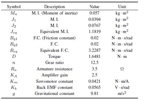
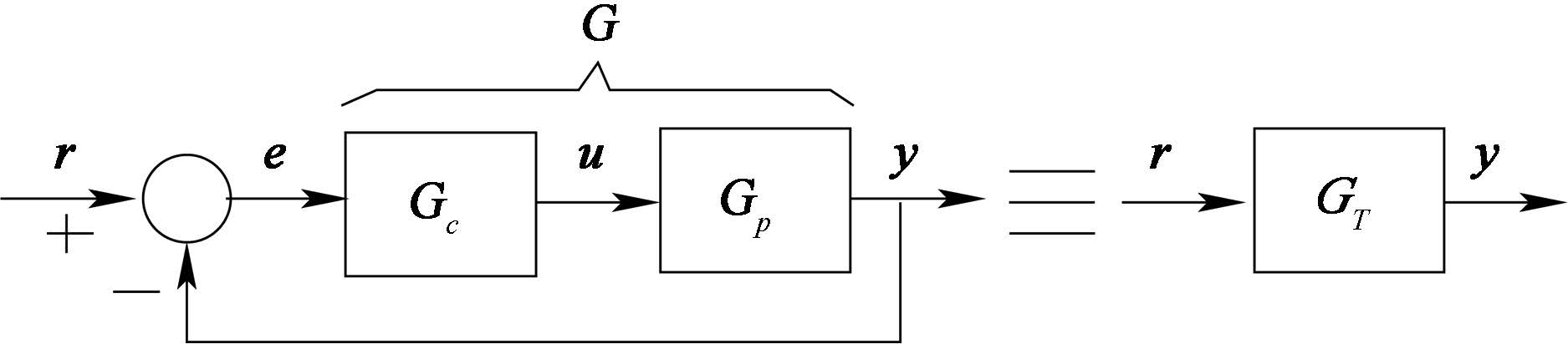
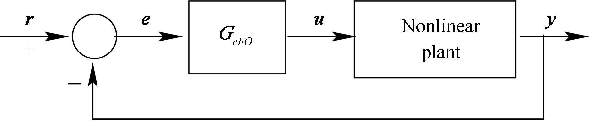
This paper develops an approach to control stable and unstable nonlinear MIMO square plants using MIMO FO controllers. The design procedure employs the LTI state space representation of the nonlinear model of the the plant. Fig. 1 depicts the linear feedback control system, where the TM function ${G}_p(s)$ of the plant is computed from its space state description. A selected diagonal closed-loop TM function denoted as ${G}_T(s)$ ensures decoupling between inputs. For design purposes, each element of this TM function has the form of a first order TF with unity gain. The step response of this TF constitutes the desired output response of the variable under control. Knowing ${G}_p(s)$ and ${G}_T(s)$, the MIMO controller ${G}_c(s)$, actually the structure of the FO MIMO controller ${G}_{cFO}(s)$ shown in Fig. 2, can be easily computed. The elements of ${G}_c(s)$ could be either transfer functions or gains. Replacing each TF of ${G}_c(s)$ with its corresponding FO TF, ${G}_c(s)$ becomes ${G}_{cFO}(s)$. For instance, the FO form of the Laplace variable $s$ is $s^{\delta}$, while the FO form of $s^{-1}$ is $s^{-\lambda}$, where $\delta$ and $\lambda$ are fractional numbers between 0 and 1. The validity of the developed design approach was verified via experimentation using the FO nonlinear control system of Fig. 2. Two applications were performed for such a purpose: control of the angular positions of a manipulator, and control of the car and arm positions of a translational manipulator.

|
Download:
|
| Fig. 1 Block diagram of the linear feedback control system. | |

|
Download:
|
| Fig. 2 Block diagram of the nonlinear FO feedback control system. | |
The MIMO FO controller designed in this work is novel due to its abilities to control not only MIMO stable plants but also nonlinear MIMO unstable ones. On the other hand, the developed approach was verified not only via simulation, but also by means of two real-time applications.
This paper is organized as follows. Section II deals with the design of the MIMO FO controller for MIMO nonlinear pla-nts. The first and second applications are described in Sections III and IV, respectively, while in Section V, some conclusions derived from this work are presented and discussed.
Ⅱ. DESIGN OF THE MIMO FO CONTROLLERA MIMO nonlinear plant can be described by the following steady state representation
| \begin{equation} \label{eq:1} \dot{X}={f}({X}, {U}), \end{equation} | (1) |
where ${f}$ is the function vector that describes the system dynamics. ${X}$ and ${U}$ are the state and control vectors, respectively. All vectors and functions are of known order. The corresponding LTI state-model can be obtained by linearization of (1) about a nominal trajectory. That is
| \begin{equation} \label{eq:2} \dot{{x}}={Ax}+{Bu}, \qquad {y}={Cx}, \end{equation} | (2) |
where ${A}$, ${B}$, and ${C}$ are the state, control and output matrices, respectively, and ${y}$ is the output vector. The TM function of the linear plant (2) is obtained from
| \begin{equation} \label{eq:3} {G}_p(s)={C}(s{I}-{A})^{-1}{B}+{D}. \end{equation} | (3) |
In (3), ${I}$ is the identity matrix and all vectors and matrices are of known orders. Fig. 1 depicts the block diagram of the MIMO LTI control system, where ${G}_c(s)$ is the MIMO controller, ${G}(s)$ is the open-loop matrix function
| \begin{equation} \label{eq:4} {G}(s)={G}_p(s){G}_c(s), \end{equation} | (4) |
${G}_T(s)$ is the closed-loop matrix function
| \begin{equation} \label{eq:5} {G}_T(s)=[{G}(s)+{I}]^{-1}{G}(s), \end{equation} | (5) |
and ${r}$, ${e}$, ${u}$ and ${y}$ represent reference, error, control and output vectors, respectively.
Consider the following diagonal closed-loop matrix function to ensure complete decoupling between different $m$ inputs
| \begin{equation} \label{eq:6} {G}_T(s)= \left[\begin{array}{ccc} G_{T11} & & \\ & \ddots & \\ & & G_{Tmm} \end{array} \right]. \end{equation} | (6) |
From (5)
| \begin{equation} \label{eq:7} {G}(s)={G}_T(s)[{I}-{G}_T(s)]^{-1}. \end{equation} | (7) |
Since ${G}_T$ is diagonal, $[{I}-{G}_T]$ and $[{I}-{G}_T]^{-1}$ are also diagonal matrices. Therefore, matrix ${G}$ takes on the diagonal form
| \begin{equation} \label{eq:8} {G}(s)= \left[\begin{array}{ccc} \frac{G_{T11}}{1-G_{T11}} & & \\ & \ddots & \\ & & \frac{G_{Tmm}}{1-G_{Tmm}} \end{array} \right]. \end{equation} | (8) |
From Fig. 1, ${y}(s)={G}_T(s){r}(s)$, where ${r}(s)$ is the reference vector. The system error ${e}(t)$ is given by
| \begin{equation} \label{eq:9} {e}(s)={r}(s)-{y}(s)= [{I}-{G}_T(s)]{r}(s). \end{equation} | (9) |
The necessary condition to make ${e}(t)$=0 in (9) is
| \begin{equation} \label{eq:10} \underset{s\to 0}{\lim}{G}_T(s)={I}. \end{equation} | (10) |
Introducing condition (10) in (5) results
| \begin{equation} \label{eq:11} {I}+{G}(0)={G}(0). \end{equation} | (11) |
This requirement means that each element of the diagonal matrix ${G}$ must contain at least one integrator. Using (4) in (5), we obtain the MIMO controller ${G}_c(s)$ depicted in Fig. 1. That is
| \begin{equation} \label{eq:12} {G}_c(s)=[{G}_p(s)]^{-1}{G}_T(s)[{I}-{G}_T(s)]^{-1}. \end{equation} | (12) |
Elements of ${G}_c(s)$ can be either gains or TF of the form
| \begin{equation} \label{eq:13} K_c;\quad \ \frac{K_i}{s};\quad \ K_ds; \quad \ {G}_x(s)=K\frac{\overset{M}{ \underset{i=0}{\Pi} }(s+z_i) } { \overset{N}{ \underset{j=0}{\Pi} }(s+p_j) }, \end{equation} | (13) |
where $Kc$, $K_i$, $K_d$ and $K$ are real gains, and $z_i$ and $p_j$ are poles and zeros of ${G}_x(s)$. Note in (13) that ${G}_x(s)$ is the general form of a TF. To formulate the FO MIMO controller denoted as ${G}_{cFO}$, terms $\frac{K_i}{s}$ and $K_ds$ of (13) are written as
| \begin{equation} \label{eq:14} \frac{K_i}{s^{\lambda}};\qquad K_ds^{\delta}, \end{equation} | (14) |
where $\delta$ and $\lambda$ are positive fractional numbers. It is worth mentioning that intensive research is performed in finding the FO counterpart of the TF ${G}_x(s)$ of (13). For example, a particular case of ${G}_x(s)$ is the following lead or lag compensator
| \begin{equation} \label{eq:15a} K\frac{(1+s/\omega_b)}{(1+s/\omega_h)}. \end{equation} | (15) |
The corresponding FO counterpart of (15) is written as[9]
| $K{{\left( \frac{1+s/{{\omega }_{k}}}{1+s/{{\omega }_{h}}} \right)}^{r}}\approx K\overset{N}{\mathop{\underset{k=0}{\mathop{\Pi }}\, }}\, \text{ }\left( \frac{1+s/{{\omega }^{\prime }}_{k}}{1+s/{{\omega }_{h}}} \right), $ |
where $0<\omega_b<\omega_h$, $K>0$, and, $\omega_k$ and $\omega^{'}_k$ are corner frequencies that are computed recursively. Fig. 2 depicts the block diagram of the FO feedback control system.
For real-time implementation, it is required to have the discrete form of the controller ${G}_{cFO}$. The discretization method by Muir's recursion[10] establishes
| \begin{equation} \label{eq:16} s^{\delta}\approx\left(\frac{2}{T}\right)^{\delta} \frac{A_n(z^{-1}, \delta)}{A_n(z^{-1}, -\delta)}, \end{equation} | (16) |
where $T$ is the sample time. In (16), polynomials $A_n(z^{-1}, \delta)$ and $A_n(z^{-1}, -\delta)$ can be computed in recursive form from
| \begin{eqnarray} &A_n(z^{-1}, \delta)= A_{n-1}(z^{-1}, \delta)-c_nz^{-n}A_{n-1}(z, \delta), \nonumber\\ &A_0(z^{-1}, \delta)= 1, ~~~~~~~~~~~~~~~~~~~~~~~~~~~~~~~~~~~~~~\nonumber\\ &\quad~~ c_n= \begin{cases} \delta/n, ~~~~~~~~ \text{if $n$ is odd}, \\ 0, ~~~~~~~~~~~ \text{if $n$ is even}. \end{cases} \label{eq:17} \end{eqnarray} | (17) |
For $n$ = 3, (17) takes on the form
| \begin{eqnarray} &A_3(z^{-1}, \delta)=-\frac{1}{3}\delta z^{-3} +\frac{1}{3}\delta^{2}z^{-2}-\delta z^{-1}+1, ~~~~~\nonumber\\ & A_3(z^{-1}, -\delta)=\frac{1}{3}\delta z^{-3} +\frac{1}{3}\delta^{2}z^{-2}+\delta z^{-1}+1.~~~~~ \label{eq:18} \end{eqnarray} | (18) |
The developed design procedure will be validated experimentally with two applications described below.
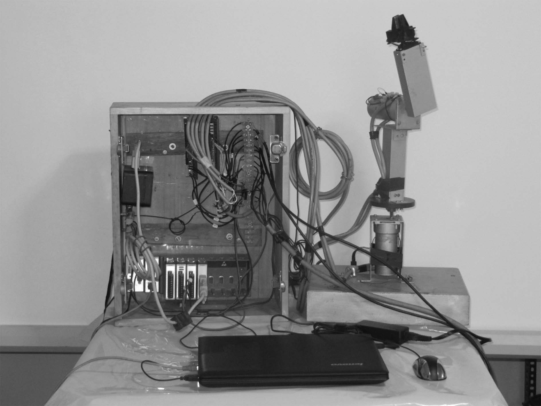
Ⅲ. FIRST APPLICATIONBase position $q_1$ and arm position $q_2$ of a manipulator of 2DOF (2 degrees of freedom) will be controlled using a MIMO FO controller. Fig. 3 shows the experimental setup. The base and the arm of the manipulator are driven by two DC servomotors having reduction mechanism and quadrature encoder to sense angular positions. A NI cRIO-9073 (Compact reconfigurable input/output) device was employed to embed the MIMO FO controller. Modules NI 9263 and NI 9401 were used to acquire angular positions and generate the control signals, respectively. Such signals were amplified using two PWM (Pulse width modulation) Galil motion control amplifiers.

|
Download:
|
| Fig. 3 The experimental setup of the manipulator of 2DOF. | |
The following dynamic model of the manipulator was obtained using Lagrange equations
| \begin{equation} \label{eq:19} {M}({q}){\ddot{q}}+{P}({q}, {\dot{q}}) {\dot{q}}+{d}({q})={u}, \end{equation} | (19) |
| \begin{align*} {M}&=\left[\begin{array}{cc} M_{11}&0 \\ 0& M_{22} \end{array}\right], \qquad {P}= \left[ \begin{array}{cc}P_{11}& P_{12}\\ P_{21}& P_{22} \end{array}\right], \nonumber\\ {d}&=\left[\begin{array}{c}0\\ d_{21} \end{array}\right], \qquad {q}=\left[\begin{array}{c} q_1\\ q_2 \end{array}\right], \qquad {u}=\left[\begin{array}{c}u_1\\u_2\end{array}\right], \nonumber \end{align*} |
| \begin{align*} &M_{11}= \frac{R_a }{nK_mK_A}\left(J_1+J_{eq}+2M_a \sin ^2 q_2\right), \nonumber\\ &M_{22}= \frac{R_a }{nK_mK_A}\left(J_2+J_{eq}\right), \nonumber\\ &P_{11}= \frac{R_a }{nK_mK_A}\left(B_{eq}+B_{q1}+\frac{n^2K_mK_b}{R_a}\right), \nonumber\\ &P_{12}= \frac{R_a }{nK_mK_A}\left(4M_a\dot{q}_1 \sin q_2\cos q_2 \right), \nonumber\\ &P_{21}= -\frac{R_a }{nK_mK_A}\left(2M_a\dot{q}_1 \sin q_2\cos q_2 \right), \nonumber\\ &P_{22}= \frac{R_a }{nK_mK_A}\left(B_{eq} + B_{q2}+\frac{n^2K_mK_b}{R_a}\right), \nonumber \\ &d_{21}= -\frac{R_a }{nK_mK_A}\left(\sin q_2 \right). \nonumber \end{align*} |
In (19), ${M}={M}^{\rm T}$ is the diagonal inertia matrix, matrices ${P}$ and ${d}$ contain Coriolis and centripetal forces, and gravitational torques, respectively. ${u}$ represents the control vector. Table I describes the valued parameters.
|
|
Table Ⅰ VALUED PARAMETERS OF THE MANIPULATOR |
Using in (19) the approximations: $\sin ^2 q_2\approx q_2^2\approx 0$, $\dot{q}_1 \sin q_2\cos q_2\approx \dot{q}_1 q_2 \approx 0$, $\sin q_2 \approx q_2$, we obtain
| \[ \overline{{M}}=\left[\begin{array}{cc}\overline{M}_{11}&0 \\ 0& \overline{M}_{22} \end{array}\right], \ \overline{{P}}= \left[\begin{array}{cc}\overline{P}_{11}& \overline{P}_{12}\\ \overline{P}_{21}& \overline{P}_{22} \end{array}\right], \ \overline{{d}}=\left[\begin{array}{c}0\\ \overline{d}_{21}q_2 \end{array}\right], \\ \] \begin{equation} \label{eq:20} \end{equation} | (20) |
| \begin{align*} \overline{M}_{11}&= \frac{R_a }{nK_mK_A}\left(J_1+J_{eq}\right), \quad \overline{M}_{22}= M_{22}, \nonumber\\ \overline{P}_{11}&= P_{11}, \quad \overline{P}_{12}= 0, \quad \overline{P}_{21}= 0, \quad \overline{P}_{22} = P_{22}, \nonumber\\ \overline{d}_{21}&= -\frac{R_a }{nK_mK_A}. \nonumber \end{align*} |
Defining as state variables: $x_1 = q_1$, $x_2 = q_2$, $x_3 = \dot{q}_1$, and $x_4 = \dot{q}_2$, the linear model (20) can be transformed into
| \begin{equation} \label{eq:21} \dot{{x}}={Ax}+{Bu}, \qquad\qquad {y}={Cx}, \end{equation} | (21) |
| \[{A}=\left[\begin{array}{cccc} 0&0&1&0\\0&0&0&1\\0&0& a_{33}&0\\ 0&a_{42}&0& a_{44}\end{array} \right], \quad {B}=\left[\begin{array}{cc} 0&0\\0&0\\ \frac{1}{\overline{M}_{11}}&0\\ 0& \frac{1}{\overline{M}_{22}} \end{array} \right] \] \[ {C}=\left[\begin{array}{cccc} 1&0&1&0\\0&1&0&0 \end{array} \right] \] |
| \begin{align} a_{33}&=-\frac{\overline{P}_{11}}{\overline{M}_{11}}, \quad a_{42}=-\frac{\overline{d}_{21}}{\overline{M}_{22}}, \quad a_{44}=-\frac{\overline{P}_{22}}{\overline{M}_{22}}, \nonumber\\ b_{31}&=-\frac{1}{\overline{M}_{11}}, \quad b_{42}=-\frac{1}{\overline{M}_{22}} \label{eq:21a} \end{align} | (22) |
It is not difficult to demonstrate that outputs of models given by (19) and (21) have unstable step responses. In order to satisfy condition (10), matrix ${G}_T(s)$ is selected as
| \begin{equation} \label{eq:22} {G}_T(s)=\left[\begin{array}{cc} \frac{1}{1+sT_1}&0\\0&\frac{1}{1+sT_2} \end{array} \right], \end{equation} | (23) |
where $T_1$ and $T_2$ are the chosen time constants of the controlled variables $q_1$ and $q_2$. Substituting (23) into (7), we obtain
| \begin{equation} \label{eq:23} {G}(s)=\left[\begin{array}{cc} \frac{1}{sT_1}&0\\0&\frac{1}{sT_2} \end{array} \right]. \end{equation} | (24) |
Observe that ${G}(s)$ in (24) meets requirement (11).
Note that ${G}_T(s)$ matrices having diagonal elements as
| \[\frac{\overset{M}{\mathop{\underset{i=0}{\mathop{\Pi }}\, }}\, ({{T}_{i}}s+1)}{\overset{N}{\mathop{\underset{j=0}{\mathop{\Pi }}\, }}\, ({{T}_{j}}s+1)}\] |
fulfill condition (10) but not requirement (11). Therefore, such matrices can not be employed to calculate the controller ${G}_c(s)$ using (12).
On the other hand, step responses of first order transfer functions as used in (23) constitute a good measure of design specifications to be met by the controlled outputs, because those show no overshoot, null steady state error, and time constants that are about one quarter of the settling times of the outputs under control.
${G}_p(s)$ and ${G}_c(s)$ matrices are obtained using equations (3) and (12), respectively. The controller ${G}_c(s)$ has the form
| \begin{equation} \label{eq:24} {G}_c(s)=\left[\begin{array}{cc} K_{c11}+K_{d11}s & 0\\ 0 & K_{c22}+K_{d22}s+\frac{K_{i22}}{s} \end{array} \right]. \end{equation} | (25) |
Parameters in (25) are function of those of (22). The corresponding FO controller is expressed as
| \begin{align} {G}_{cFO}(s)&= \left[\begin{array}{cc} K_{c11}+K_{d11}s^{\delta} & 0\\ 0 & K_{c22}+K_{d22}s^{\delta}+\frac{K_{i22}}{s^{\lambda}} \end{array} \right].\nonumber\\ & \label{eq:25} \end{align} | (26) |
From Fig. 2, the FO control force is described by
| \begin{equation} \label{eq:26} {u}(s)={G}_{cFO}(s){e}(s). \end{equation} | (27) |
Substituting (16) with $n$ = 3 into (26), and using the shift property $z^{-n}u_i(z)=u_i(k-n)$ and $z^{-n}e_i(z)=e_i(k-n)$, $i$ = 1, 2, where $k$ is the discrete time, we obtain the following difference equations for the control forces
| \begin{align} u_1(k)&=\frac{1}{a_0}\left[-\overset{6}{\underset{i=1}{\Sigma}} a_iu_1(k-i)+ \overset{6}{\underset{j=0}{\Sigma}} b_je_1(k-j)\right], \nonumber\\ u_2(k)&=\frac{1}{a_0}\left[-\overset{6}{\underset{i=1}{\Sigma}} a_iu_2(k-i)+ \overset{6}{\underset{j=0}{\Sigma}} h_je_2(k-j)\right ].\label{eq:27} \end{align} | (28) |
In (28), all $a_i$, $b_j$ and $h_j$ are known constants, for instance
| \begin{align*} a_6 &= - \delta\lambda, \qquad a_0=1, \nonumber\\ b_6&= \frac{1}{9} K_{d11}\delta\lambda(\frac{2}{T})^\delta - \frac{1}{9}K_{c11}\delta\lambda , \nonumber\\ h_6&= \frac{1}{9}K_{d22}\delta\lambda(\frac{2}{T})^\delta-\frac{1}{9}K_{c22}\delta\lambda - \frac{1}{9}K_{i22}\delta\lambda(\frac{2}{T})^{-\lambda}, \nonumber \end{align*} |
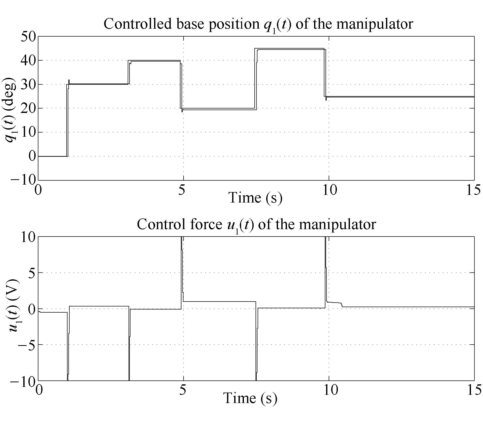
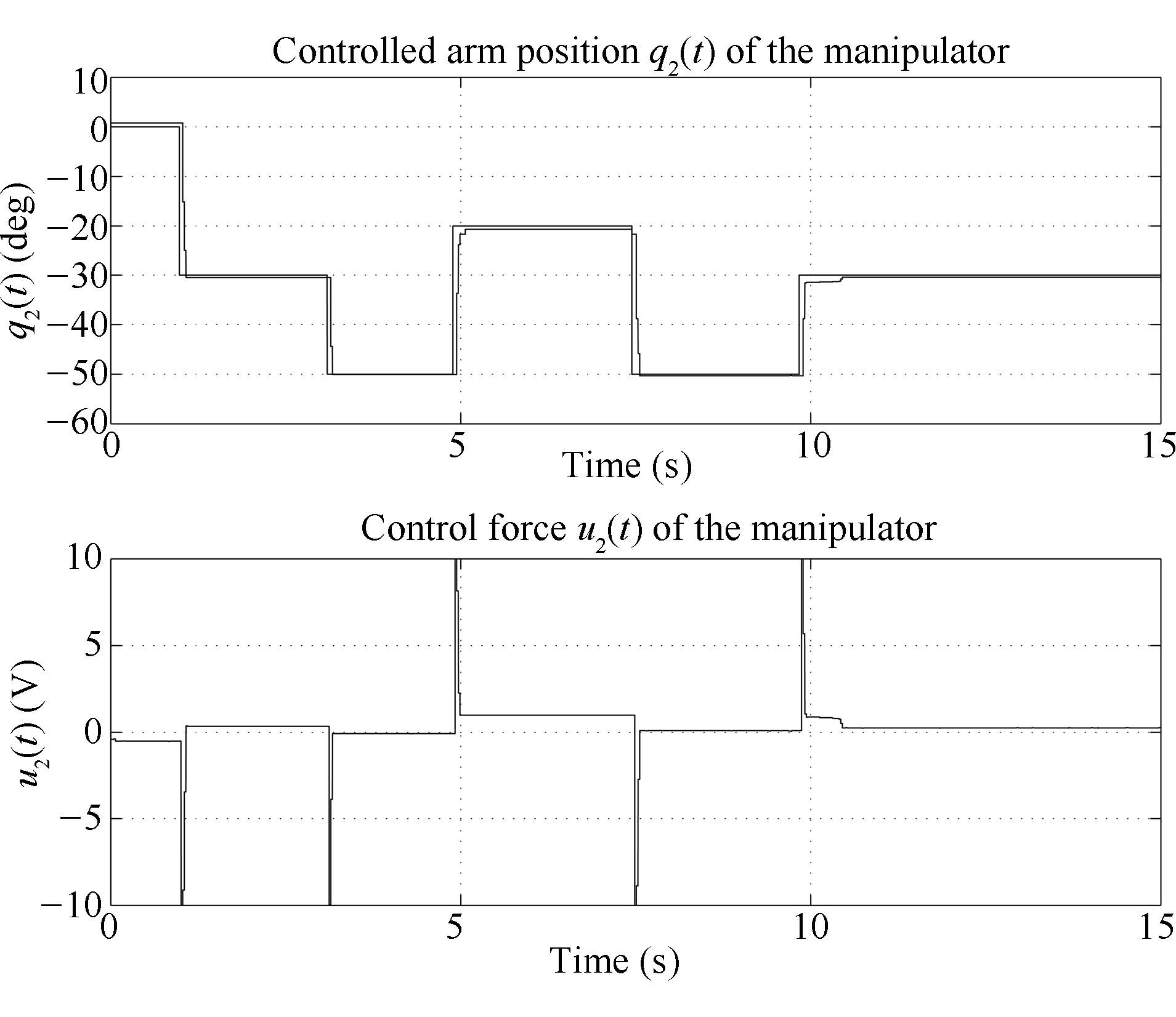
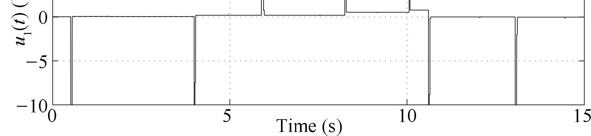
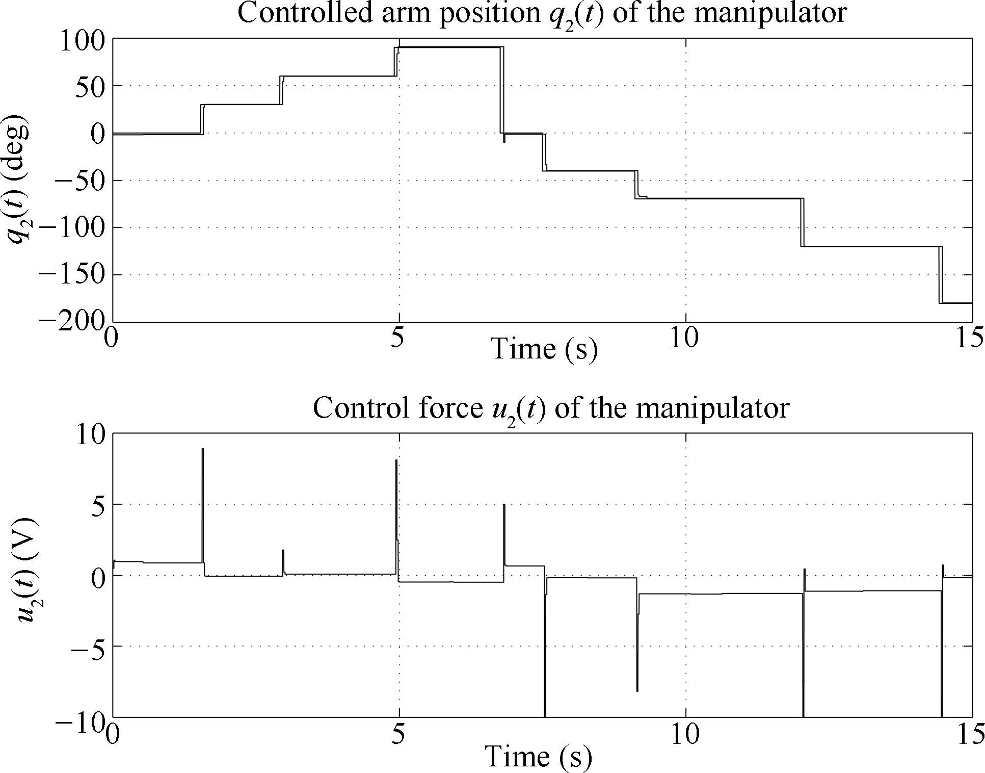
where $T$ is the sampling time selected as 1 ms in this work. The FO control system was simulated in Mathscript with time constants $T_1$ and $T_2$ and FO parameters $\delta$ and $\lambda$ set to 0.5, 0.5, 0.5 and 0.9, respectively. The other gains were taken from (25): $K_{c11}$ = 10.7, $K_{d11}$ = 0.866, $K_{c22}$ = 26.74, $K_{d22}$ = 4.66, $K_{i22}$ = $-$13.2786. For the experimentation phase, $K_{c11}$ was set to 15. Fig. 4 and Fig. 5 depict the experimental results.

|
Download:
|
| Fig. 4 Controlled base position $q_1(t)$ of the manipulator with respect to step wise references. | |

|
Download:
|
| Fig. 5 Controlled arm position $q_2(t)$ of the manipulator with respect to step wise references. | |
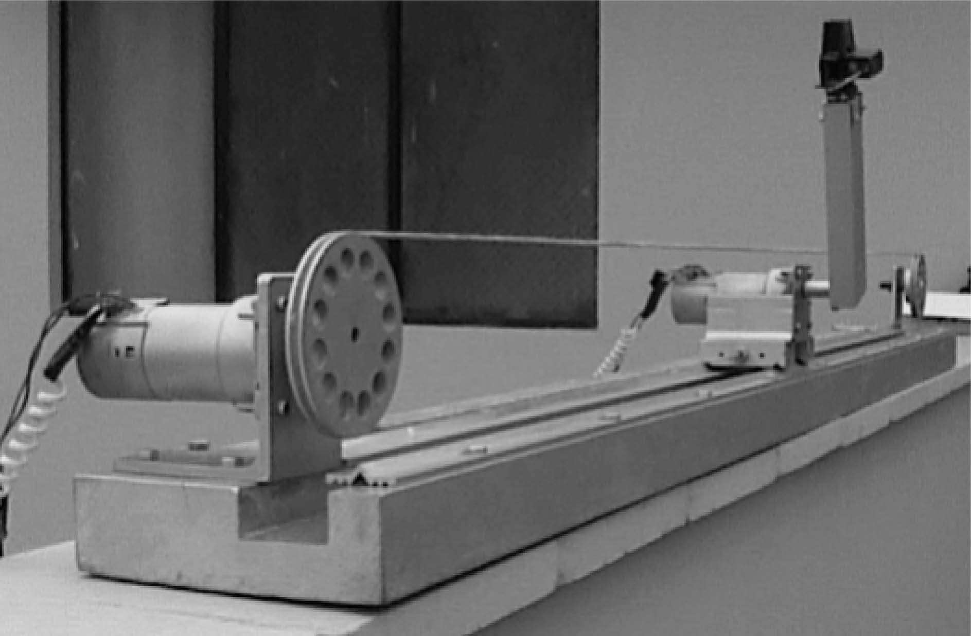
The linear position $q_1$ of the car and the angular position $q_2$ of the arm of a translational manipulator of 2DOF shown in Fig. 6 will be controlled with a MIMO FO controller. The manipulator possesses two DC servomotors with reduction mechanism and quadrature encoders to sense angular positions. One servomotor is attached to the axis of one of the two pulleys. Those pulleys carry a cable to transmit the force to translate the car, which is mounted on rails. The other servomotor is mounted on the car to drive the arm. This application uses the same experimental setup as the first one.

|
Download:
|
| Fig. 6 The translational manipulator of 2DOF. | |
The dynamic model of the manipulator was also obtained employing Lagrange equations. The resulting nonlinear model takes on the form
| \begin{equation} \label{eq:28} {M}({q})\ddot{{q}}+{P}({q}, \dot{{q}}) \dot{{q}}+ {d}({q})={u} \end{equation} | (29) |
| \[{q}=\left[\begin{array}{c} q_1\\ q_2 \end{array}\right]= \left[\begin{array}{c} r\\ \theta \end{array}\right], \qquad {u}=\left[\begin{array}{c}u_1\\u_2\end{array}\right], \qquad {d}=\left[\begin{array}{c}0\\d_{21} \end{array}\right], \] |
| \[ {M}=\left[\begin{array}{cc}M_{11}&M_{12}\\ M_{21}&M_{22} \end{array}\right], \quad\quad {P}= \left[ \begin{array}{cc}P_{11}&P_{12}\\0& P_{22}\end{array}\right], \quad\quad \] |
| \begin{align*} M_{11}&=\frac{J_x+m_1}{K_xK_{A1}}, \qquad\qquad\qquad M_{12}= \frac{m_2}{K_xK_{A1}}\cos\theta, \nonumber\\ M_{21}&=\frac{m_2}{r_p K_xK_{A2}}\cos\theta, \qquad \ \ \ M_{22}=\frac{J_{eq2}+J_t}{r_pK_xK_{A2}}, \nonumber\\ P_{11}&=\frac{B_x+B_F}{K_xK_{A1}}, \qquad\qquad\quad P_{12}= -\frac{m_2}{K_xK_{A1}}\dot{\theta} \sin \theta, \nonumber\\ P_{22}&= \frac{\frac{n^2K_mK_b}{Ra}+B_{eq2}+B_{T}}{r_pK_xK_{A2}}, \nonumber\\ d_{21}&=-\frac{gm_2}{r_pK_xK_{A2}} \sin\theta. \nonumber \end{align*} |
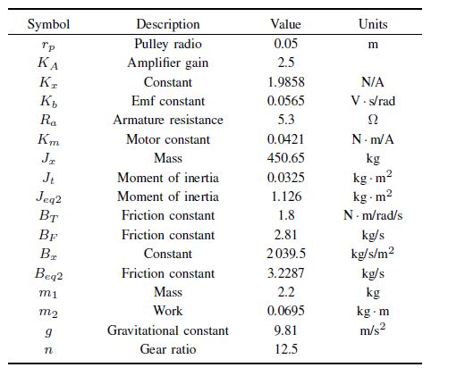
Observe that matrix ${M}$ in (29) is neither diagonal nor symmetric which makes the manipulator more challenging to be controlled. Recall that matrix ${M}$ in (20) was diagonal. Table II describes the valued parameters of the translational manipulator.
|
|
Table Ⅱ VALUED PARAMETERS OF THE MANIPULATOR |
On using the approximations $\cos \theta \approx 1$, $\sin \theta \approx \theta$ and $\dot{\theta}\sin \theta \approx 0$ in (29), we obtain
| \begin{align} \overline{M}_{11}&=M_{11}, \ \ \quad \overline{M}_{12}= \frac{m_2}{K_xK_{A1}}, \ \ \quad \overline{M}_{21}=\frac{m_2}{r_p K_xK_{A2}}, \nonumber\\ \overline{M}_{22}&= M_{22}, \ \ \quad \overline{P}_{11}=P_{11}, \ \ \quad \overline{P}_{12}= 0, \ \ \quad \overline{P}_{22}= P_{22}, \nonumber\\ \overline{d}_{21}&=-\frac{gm_2}{r_pK_xK_{A2}}. \label{eq:29} \end{align} | (30) |
Defining as state variables: $x_1=r$, $x_2=\theta$, $x_3=\dot{r}$ and $x_4=\dot{\theta}$, the nonlinear model of (29) using (30) can be transformed into the following state equation
| \begin{equation} \label{eq:30} \dot{{x}}={Ax}+{Bu}, \qquad\qquad {y}={Cx}, \end{equation} | (31) |
| \[{A}=\left[\begin{array}{cccc} 0&0&1&0\\0&0&0&1\\0&a_{32}& a_{33}&a_{34}\\ 0&a_{42}&a_{43}& a_{44}\end{array} \right], \quad {B}=\left[\begin{array}{cc} 0&0\\0&0\\ b_{31}&b_{32}\\ b_{41}& b_{42} \end{array} \right], \] |
| \[ {C}=\left[\begin{array}{cccc} 1&0&1&0\\0&1&0&0 \end{array} \right], \] |
| \begin{align} a_{32}&=\frac{\overline{M}_{12}\overline{d}_{21}}{\overline{den}}, \qquad a_{33}=-\frac{\overline{M}_{22}\overline{P}_{11}}{\overline{den}}, \nonumber\\ a_{34}&=\frac{\overline{M}_{12}\overline{P}_{22}}{\overline{den}}, \qquad a_{42}=-\frac{\overline{M}_{11}\overline{d}_{21}}{\overline{den}}, \nonumber\\ a_{43}&=\frac{\overline{M}_{21}\overline{P}_{11}}{\overline{den}}, \qquad a_{44}=-\frac{\overline{M}_{11}\overline{P}_{22}}{\overline{den}}, \nonumber\\ b_{31}&=\frac{\overline{M}_{22}}{\overline{den}}, \ \ \quad\qquad b_{32}=-\frac{\overline{M}_{12}}{\overline{den}}, \nonumber\\ b_{41}&=-\frac{\overline{M}_{21}}{\overline{den}}, \qquad\quad b_{42}=\frac{\overline{M}_{11}}{\overline{den} }, \nonumber\\ \overline{den}&=\overline{M}_{11}\overline{M}_{22}-\overline{M}_{12}\overline{M}_{21}. \label{eq:30a} \end{align} | (32) |
It is not difficult to prove that outputs of models given by (29) and (31) possess unstable step responses. According to (10), ${G}_T(s)$ matrix is chosen as in (23). ${G}_p(s)$, ${G}_c(s)$ and ${G}(s)$ matrices are obtained using (3), (12) and (4), respectively. ${G}(s)$ results in a matrix that has the same form as (24). The ${G}_c(s)$ matrix is calculated using relation (12)
| \begin{equation} \label{eq:31} {G}_c(s)=\left[\begin{array}{cc} K_{c11}+K_{d11}s & K_{c12}+\frac{K_{i12}}{s}+ K_{d12}s\\ \\ K_{c21}+K_{d21}s & K_{c22}+\frac{K_{i22}}{s}+K_{d22}s \end{array} \right]. \end{equation} | (33) |
Parameters of (33) are function of parameters described in (32). The corresponding FO controller is expressed as
| \begin{eqnarray} &{G}_{cFO}(s)\quad\quad\quad\quad \quad\quad\quad\quad\quad\quad\quad\quad\quad\quad\quad\quad\quad\quad\nonumber\\ & =\left[\begin{array}{cc} K_{c11}+K_{d11}s^{\delta} & K_{c12}+ \frac{K_{i12}}{s^{\lambda}}+ K_{d12}s^{\delta}\\ \\ K_{c21}+K_{d21}s^{\delta} & K_{c22}+ \frac{K_{i22}}{s^{\lambda}}+K_{d22}s^{\delta} \end{array} \right]. \label{eq:32} \end{eqnarray} | (34) |
Compare (33) with (25) and (34) with (26). Replacing (16) with $n$ = 3 in (34), and then employing the shift property, we obtain the following difference equations for the vector control (27)
| \begin{align} u_1(k)&=\frac{1}{a_0}\left[-\overset{6}{\underset{i=1}{\Sigma}} a_iu_1(k-i)+ \overset{6}{\underset{j=0}{\Sigma}} b_je_1(k-j)\right . \nonumber\\ & \left. +\overset{6}{\underset{j=0}{\Sigma}} c_je_2(k-j)\right], \nonumber\\ u_2(k)&=\frac{1}{a_0}\left[-\overset{6}{\underset{i=1}{\Sigma}} a_iu_2(k-i)+ \overset{6}{\underset{j=0}{\Sigma}} g_je_2(k-j) \right .\nonumber\\ &+\left. \overset{6}{\underset{j=0}{\Sigma}} h_je_2(k-j)\right]. \label{eq:33} \end{align} | (35) |
In (35), $k$ is the discrete time, and all $a_i$, $b_j$ and $h_j$ are known constants as in (27). $T$, the sampling time, was selected to be 1 ms. The FO control system for this manipulator was simulated in Mathscript with time constants $T_1$ and $T_2$ and FO parameters $\delta$ and $\lambda$ set to 0.3, 0.5, 0.6 and 0.75, respectively. The other gains were taken from (31): $K_{c11}$ =220, $K_{d11}$ = 1, $K_{c12}$ = 0, $K_{i12}$ = 0; $K_{d12}$ = 0.028, $K_{c21}$ = 0, $K_{d21}$ = 0.0093, $K_{c22}$ = 20, $K_{d22}$ = 10, $K_{i22}$ = $-$5. For the experimentation phase, $K_{c11}$ was set to 25. Fig. 7 and Fig. 8 depict the experimental results.

|
Download:
|
| Fig. 7 Controlled car position $q_1(t)$ of the manipulator with respect to step wise references. | |

|
Download:
|
| Fig. 8 Controlled arm position $q_2(t)$ of the manipulator with respect to step wise references. | |
In light of the results in Sections III and IV, the main goal of this work has been achieved: experimental verification of the design approach to control nonlinear MIMO processes using MIMO FO controllers.
The nonlinear model of the plant is necessary to obtain the linear model required to design the structure of the FO controller, and to test via simulation the designed FO controller. In the simulation phase, controller parameters were tuned using the trial and error method. Such valued parameters were used with few modifications for the experimentation phase.
Intensive work has been done in tuning rules development for FO SISO (Single-input single-output) controllers. It is still under research to extend the results for FO MIMO controllers. No tuning methods for controllers of the forms given by (26) and (34) have been reported. Moreover, depending on the application, the structure of a FO MIMO controller can change (compare (26) with (34)), making the development of proper tuning rules difficult. For such reasons, this work employed the trial and error method.
MIMO FO controllers designed in [4, 6], and [7] were tuned using different methods, because such controllers have diagonal forms with each diagonal element being a FO SISO controller.
This work is novel because unlike others the designed FO MIMO controller can be applied not only to stable MIMO plants, but also to nonlinear unstable MIMO plants. This approach was tested not only via simulation but also via experimentation.
The proposed design procedure can also be applied to MIMO time-delay plants. In order to obtain a LTI state space description of the plant, TF containing time-delays need to be replaced by equivalent TF. For example[11]
| \[\frac{1}{2s+1}{\rm e}^{-2s} \approx \frac{1}{(s+1)^{4}}\] |
It is necessary to perform more research related to the design of a FO MIMO controller when the structure of the controller, matrices (25) and (33) for example, has terms of the form
| \[G_x(s)=K\frac{\overset{M}{ \underset{i=0}{\Pi} }(s+z_i) } { \overset{N}{ \underset{j=0}{\Pi} }(s+p_j) }\] |
| [1] | Karad S, Chatterji S, Suryawanshi P. Performance analysis of fractional order PID controller with the conventional PID controller for bioreactor control. International Journal of Scientific&Engineering Research, 2012, 3(6): 1-6 |
| [2] | Singh S, Kosti A. Comparative study of integer order PI-PD controller and fractional order PI-PD controller of a DC motor for speed and position control. International Journal of Electrical and Electronic Engineering & Telecommunications, 2015, 4(2): 22-26 |
| [3] | Chen Y, Petrăš I, Xue D. Fractional order control-a tutorial. In: Proceedings of the 2009 American Control Conference. St. Louis, MO, USA: IEEE, 2009. 1397-1411 |
| [4] | Banu U S, Lakshmanaprabu S K. Multiloop fractional order PID controller tuned using cuckoo algorithm for two interacting conical tank process. World Academy of Science, Engineering and Technology, International Journal of Mechanical and Mechatronics Engineering, 2015, 2(1): 742 |
| [5] | Moradi M. A genetic-multivariable fractional order PID control to multiinput multi-output processes. Journal of Process Control, 2014, 24(4): 336-343 |
| [6] | Sivananaithaperumal S, Baskar S. Design of multivariable fractional order PID controller using covariance matrix adaptation evolution strategy. Archives of Control Sciences, 2014, 24(2): 235-251 |
| [7] | Muresan C I, Dulf E H, Ionescu C M. Multivariable fractional order PI controller for time delay processes. In: Proceedings of the 2012 International Conference on Engineering and Applied Science. Colombo, Sri Lanka, 2012. |
| [8] | Song X N, Chen Y Q, Tejado I, Vinagre B M. Multivariable fractional order PID controller design via LMI approach. In: Proceedings of the 18th IFAC World Congress. Milano, Italy: IFAC, 2011. 13960-13965 |
| [9] | Malti R, Melchior P, Lanusse P, Oustaloup A. Towards an object oriented CRONE toolbox for fractional differential systems. In: Proceedings of the 18th IFAC World Congress. Milano, Italy: IFAC, 2011. 10830-10835 |
| [10] | Vinagre B M, Chen Y Q, Petrăš I. Two direct Tustin discretization methods for fractional-order differentiator/integrator. Journal of the Franklin Institute, 2003, 340(5): 349-362 |
| [11] | Michalowski T. Applications of MATLAB in Science and Engineering. Rijeka, Croatia: InTech, 2011. |