 2016, Vol.3


The orders of the adaptive laws were selected by particle swarm optimization (PSO), using an objective function including the ISI and the ISE, with different weighting factors. The results show that, when ISI index is taken into account in the optimization process to determine the orders of adaptive laws, the resulting values are fractional, indicating that control energy of the scheme might be better managed if fractional adaptive laws are used.
The main idea behind direct model reference adaptive control (direct MRAC) technique is to create a closed loop system with adjustable parameters, such that the application of the resulting control signal to the plant makes the output of the plant to follow the output of a given reference model. Adaptive laws for adjusting controller parameters have been synthesized using several techniques, where the most commonly used is the gradient approach, in which the estimated parameter is the result of a differential equation of integer order, moving in the negative direction of the gradient of the criterion function to be minimized[1].
The fractional calculus, that is calculus of integrals and derivatives of real or complex orders[2], has been increasingly used in many fields of science and engineering, and the control techniques are not the exception. Since the paper by Vinagre et al.[3], which as far as we know is the first paper proposing the inclusion of fractional operators in MRAC schemes, many works have been published including fractional operators not only in MRAC schemes (see for example [4, 5, 6, 7, 8, 9]) but also in some other adaptive schemes[10, 11]. Some researchers have mentioned advantages of using fractional operators in MRAC schemes such as better management of noise[10], better behavior under disturbances[4, 5, 9] and improvements in transient responses[3, 9], among others.
However, there is still a reticence in the adaptive control community about using these fractional operators inside adaptive schemes because of their complexity. In [9] it has been mentioned that the use of fractional adaptive laws in a MRAC scheme for an automatic voltage regulator leads to a smoother control signal, which is a very interesting fact. This behavior could be seen as a better management of the energy used in the control scheme, and this could be a point in favor of the fractional operators, at least in MRAC schemes, since energy efficiency is a trending topic nowadays due to the increasing cost of energy worldwide.
This paper makes a preliminary analysis of the behavior of control signals in a MRAC scheme, when fractional adaptive laws are used to adjust control parameters. The analysis is made empirically, since it follows from simulation studies, but we believe this could be the first step to a more detailed study on this topic. The results show that the introduction of fractional adaptive laws in the MRAC schemes analyzed leads to smoother control signals, with a lower integral of the squared control, which can be seen as a better management of the energy spent in the control scheme. The simulations also show that there could exist a trade-off between the control energy and the convergence speed of the control error, which suggests the use of optimization techniques to select the suitable orders to be used in adaptive laws.
The paper is organized as follows. Section II presents some basic concepts about fractional calculus. Section III introduces the MRAC scheme that is analyzed in the paper, with the corresponding fractional adaptive laws. Section IV presents the simulation and analysis of the results for the MRAC scheme, implemented for three different plants: one stable, one marginally stable and one unstable. Finally, Section V presents the conclusions of the study.
Ⅱ. BASIC CONCEPTSThis section presents some basic concepts of fractional calculus, which are used in this paper.
A. Fractional CalculusFractional calculus studies integrals and derivatives of real or complex orders[2]. The Riemann-Liouville fractional integral is one of the main concepts of fractional calculus, and is presented in Definition 1.
Definition 1 (Riemann-Liouville fractional integral)[2].
| \begin{equation} I_{a+}^{\alpha}f\left(t\right)=\frac{1}{\Gamma\left(\alpha\right)} \int_{a}^{t}\frac{f\left(\tau\right)}{\left(t-\tau\right)^{1-\alpha}}{\rm d}\tau, \quad t>a, \, R\left(\alpha\right)>0, \label{eq:frac_integral} \end{equation} | (1) |
where $\Gamma\left(\alpha\right)$ corresponds to the Gamma Function, given by Equation (2).
| \begin{equation} \Gamma\left(\alpha\right)=\int_{0}^{\infty}t^{\alpha-1}{\rm e}^{-t}{\rm d}t. \label{eq:Gammafun} \end{equation} | (2) |
There are several definitions regarding fractional derivatives. Definition 2 corresponds to the fractional derivative according to Caputo, and is the one used in this paper for implementing fractional adaptive laws.
Definition 2 (Caputo fractional derivative)[2].
| \begin{equation} {t_0}{C}{D}_t^\alpha x\left(t\right)=\frac{1}{\Gamma\left(n-\alpha\right)}\int_{a}^{t}\frac{f^{\left(n\right)}\left(\tau\right)}{\left(t-\tau\right)^{\alpha-n+1}}{\rm d}\tau, \label{eq:Caputo_der} \end{equation} | (3) |
where $t>a, \quad n-1<\alpha<n, \quad n\in\bf{Z}^{+}$.
Ⅲ. MODEL REFERENCE ADAPTIVE CONTROL SCHEMEIn this section, we present the structure of the MRAC scheme analyzed in this work. Since this adaptive scheme has been very well studied in [1], for the sake of space we only present here the equations needed for its implementation. For more specific details, the reader is referred to [1], Chapter 5.
A. MRAC Scheme for Plants with Only the Output AccessibleUsually, the whole state of a plant is not accessible, because some variables cannot be physically measured or because there is no instrumentation available to do it. In these cases, the designer has access only to the input and output of the plant, and the control scheme must be designed under these constraints.
Let us consider a single-input single-output linear time invariant plant of $n$-{th} order described by the vector differential equation
| \begin{equation} \begin{array}{l} \dot{x}_p\left(t\right)= A_p x_p\left(t\right)+b_p u\left(t\right), \\ y_p\left(t\right)=h_p^{\rm T} x_p\left(t\right), \end{array} \label{eq:planta_frac} \end{equation} | (4) |
where $A_p\in{\bf R}^{n\times n}$, $b_p, h_p\in{\bf R}^{n}$ are completely unknown. $x_p\in{\bf R}^n$ is the state vector, which is not accessible, and $u, y_p\in{\bf R}$ are the input and the output of the system. The plant is assumed to be controllable and observable.
An asymptotically stable reference model is specified by the linear time-invariant system described by
| \begin{equation} \begin{array}{l} \dot{x}_m\left(t\right)= A_m x_m\left(t\right)+b_m r\left(t\right), \\ y_m\left(t\right)=h_m^{\rm T} x_m\left(t\right), \end{array} \label{eq:modelo_ref_frac} \end{equation} | (5) |
where $A_m\in{\bf R}^{n\times n}$ is a known asymptotically stable matrix and $b_m, h_m\in{\bf R}^{n}$ are known vectors. The reference model is assumed to be controllable and observable. $y_m\in{\bf R}$ is the output of the reference model and $r\in{\bf R}$ is a bounded reference input. It is assumed that $y_m\!\left(t\right)$, for all $t\geq t_0$, represents the desired trajectory for $y_p\!\left(t\right)$.
The transfer function of the plant (4) can be represented as
| \begin{equation} W_p\left(s\right)=h_p^{\rm T}\left(sI-A_p\right)^{-1}b_p=k_p\frac{Z_p\left(s\right)}{R_p\left(s\right)} \label{eq:plant_tf} \end{equation} | (6) |
where $k_p$ is the high frequency gain and $Z_p\left(s\right), R_p\left(s\right)$ are monic polynomials with unknown parameters. It is assumed that $Z_p\left(s\right)$ is a Hurwitz polynomial and that the sign of $k_p$ is known. The control goal here is to keep bounded all the signals of the scheme and that ${\lim}_{t\rightarrow\infty} \left(y_p\left(t\right)-y_m\left(t\right)\right)=0$.
As we may expect, having no access to the plant state implies that a more complex control scheme has to be used in the problem to synthesize stable adaptive laws, compared to the case when the whole state $x_p\left(t\right)$ is accessible (see [1], Chapter 3). For this kind of scheme and with no loss of generality, it is assumed that the transfer function of the reference model is strictly positive real (SPR). The transfer function of the reference model is represented as
| \begin{equation} W_m\left(s\right)=h_m^{\rm T}\left(sI-A_m\right)^{-1}b_m=k_m\frac{Z_m\left(s\right)}{R_m\left(s\right)}, \label{eq:rmodel_tf} \end{equation} | (7) |
where $k_m$ is the high frequency gain and $Z_m\left(s\right), R_m\left(s\right)$ are monic coprime and Hurwitz polynomials with all the parameters known. Note that since the reference model is chosen by the designer, then all these conditions can be fulfilled.
This control problem has to be solved in a different way for plants with relative degree $n^*=1$ and for plants with relative degree ${{n}^{*}}\ge 2$[1]. For the sake of simplicity, let us consider that the plant under study has relative degree $n^*=1$. Then, the control input to the plant is chosen as
| \begin{equation} u\left(t\right)=\theta^{\rm T}\left(t\right)\omega\left(t\right), \label{eq:ley_control_noacc} \end{equation} | (8) |
where $\theta\left(t\right)\in{\bf R}^{2n}$ is a vector of adjustable parameters and $\omega\left(t\right)\in{\bf R}^{2n}$ is a vector of known signals. Specifically
| \begin{equation} \begin{array}{l} \theta\left(t\right)=\left[k\left(t\right)\quad \theta_1^{\rm T}\left(t\right)\quad \theta_0\left(t\right)\quad \theta_2^{\rm T}\left(t\right)\right]^{\rm T}, \\ \omega\left(t\right)=\left[r\left(t\right)\quad \omega_1^{\rm T}\left(t\right)\quad y_p\left(t\right)\quad \omega_2^{\rm T}\left(t\right)\right]^{\rm T}, \end{array} \end{equation} | (9) |
with $k, \theta_0:{\bf R}^+\rightarrow{\bf R};\theta_1, \omega_1:{\bf R}^+\rightarrow{\bf R}^{n-1};\theta_2, \omega_2:{\bf R}^+\rightarrow{\bf R}^{n-1}$.
The auxiliary signals $\omega_1\left(t\right)\in{\bf R}^{n-1}, \omega_2\left(t\right)\in{\bf R}^{n-1}$ are obtained by filtering the input and the output, respectively,
| \begin{equation} \begin{array}{l} \dot{\omega}_1\left(t\right)=\Lambda\omega_1\left(t\right)+l\;u\left(t\right), \\ \dot{\omega}_2\left(t\right)=\Lambda\omega_2\left(t\right)+l\;y_p\left(t\right), \end{array} \end{equation} | (10) |
where $\Lambda\in{\bf R}^{\left(n-1\right)\times\left(n-1\right)}$ and $l\in{\bf R}^{n-1}$ must be chosen such that det$\left(sI-\Lambda\right)=Z_m\left(s\right)$ and the pair $\left(\Lambda, l\right)$ is controllable and asymptotically stable.
Defining the control error as
| \begin{equation} e\left(t\right)=y_p\left(t\right)-y_m\left(t\right), \label{eq:error_no_acc} \end{equation} | (11) |
then for the classic integer order MRAC (IOMRAC) the stable adaptive laws for the parameters are generated as
| \begin{equation} \begin{array}{l} \dot{k}\left(t\right)=-\gamma\, {\rm sgn}\left(k_p\right)e\left(t\right)r\left(t\right), \\ \dot{\theta}_0\left(t\right)=-\gamma\, {\rm sgn}\left(k_p\right)e\left(t\right)y_p\left(t\right), \\ \dot{\theta}_1\left(t\right)=-\gamma\, {\rm sgn}\left(k_p\right)e\left(t\right)\omega_1\left(t\right), \\ \dot{\theta}_2\left(t\right)=-\gamma\, {\rm sgn}\left(k_p\right)e\left(t\right)\omega_2\left(t\right), \end{array} \label{eq:ajuste_ent_noacc} \end{equation} | (12) |
where $\gamma\in{\bf R}^+$ corresponds to the adaptive gain[1].
In this work we are going to use the same structure already explained for the IOMRAC scheme, but using fractional adaptive laws (FOMRAC) given by
| \begin{equation} \begin{array}{l} {C}{D}_{t_0}^{\alpha_k}k\left(t\right)=-\gamma\, {\rm sgn}\left(k_p\right)e\left(t\right)r\left(t\right), \\ {C}{D}_{t_0}^{\alpha_{0}}\theta_0\left(t\right)=-\gamma\, {\rm sgn}\left(k_p\right)e\left(t\right)y_p\left(t\right), \\ {C}{D}_{t_0}^{\alpha_1}\theta_1\left(t\right)=-\gamma\, {\rm sgn}\left(k_p\right)e\left(t\right)\omega_1\left(t\right), \\ {C}{D}_{t_0}^{\alpha_2}\theta_2\left(t\right)=-\gamma\, {\rm sgn}\left(k_p\right)e\left(t\right)\omega_2\left(t\right), \end{array} \label{eq:ajuste_frac_noacc} \end{equation} | (13) |
where $\alpha_k, \alpha_0$ and each component of $\alpha_1, \alpha_2$ belong to the interval $\left(0, 1\right]$. It is important to have in mind that these fractional orders can be different for every component of the adaptive laws.
It should also be noted that, although some advances have been made regarding the stability analysis of fractional adaptive schemes[12], the stability of this particular case has not been proved yet. Nevertheless, since the main idea of this work is obtaining some empirical conclusions from simulation studies on the control effort, we will focus only on this topic. The reader will observe, however, that in simulation studies the fractional case remains stable as well.
Ⅳ. SIMULATIONS STUDIESIn this section we will study the control of three second order plants, using the controller presented in Section III, through simulations. The plants under control have the same vectors $b_p, h_p$ specified in (14), and only the matrix $A_p$ changes from one plant to another.
In the first case we study an unstable plant ($a_{11}=4, \;a_{12}=-1, \;a_{21}=5, \;a_{22}=-3$) with poles $p_1=3.1926$ and $p_2=-2.1926$. The second case corresponds to a marginally stable plant ($a_{11}=-5, \;a_{12}=1, \;a_{21}=0, \;a_{22}=0$), with poles $p_1=0$ and $p_2=-5$. Finally, the third case corresponds to a stable plant ($a_{11}=-5, \;a_{12}=3, \;a_{21}=-15, \;a_{22}=1$) with complex conjugate poles $p_{1, 2}=-2\pm 6i$. The reference model is asymptotically stable, as detailed in (14).
| \begin{equation} \begin{array}{c} A_p=\left[\begin{array}{c c}a_{11}&a_{12}\\a_{21}&a_{22}\end{array}\right], \; A_m=\left[\begin{array}{c c}-1&0\\0&-2\end{array}\right], \\\\ b_p=b_m=\left[\begin{array}{l}1\\1\end{array}\right], \;h_p=h_m=\left[\begin{array}{l}1\\0\end{array}\right]. \end{array} \label{eq:used_plants} \end{equation} | (14) |
The initial conditions used in simulations are $x_p\left(0\right)=\left[0\;\;1\right]^{\rm T}$ and $x_m\left(0\right)=\left[1\;\;5\right]^{\rm T}$.
It can be checked that the transfer function of the reference model is SPR and the relative degree is $n^*=1$ for the three plants, so that conditions for designing MRAC are fulfilled. Since the numerator of the reference model transfer function is $Z_m\left(s\right)=s+2$, the design parameters $\Lambda, l$ were chosen as $\Lambda=-2$ and $l=1$.
For the three plants to be controlled, the initial conditions of the four estimated parameters were chosen as $\theta\left(0\right)=\left[5\;\;4 \;\;-8 \;\;-5 \right]^{\rm T}$, the simulation time was set to $T=500$ s, $\gamma=1$ and the reference input $r\left(t\right)$ used is a unit step.
As we mentioned at the beginning of this paper, we will focus on analyzing how the management of control energy can be improved using fractional adaptive laws. To that extent, we use the integral of the squared input (ISI) as an indicator of the control energy, calculated using the following expression
| \begin{equation} ISI=\int_0^T u^2\left(t\right){\rm d}t, \label{eq:isi} \end{equation} | (15) |
where $T$ is the final simulation time.
Since the control signal is usually generated using some kind of energy, then ISI represents an excellent measurement of the energy spent to control the plant. Nowadays, ISI has become extremely important in control schemes, since industrial processes design and operation are focusing on saving energy, as a way of contributing to protect natural resources and planet sustainability.
Although our main goal is showing that the use of the fractional adaptive laws may improve the use of control energy in the adaptive schemes, we have to consider another important variable which is the control error. The integral of the squared control error is usually used as a performance index, measuring the deviation of the controlled variable from its desired value over the time. This index is given in (16) and it will be taken in mind during our studies as well.
| \begin{equation} ISE=\int_0^T e^2\left(t\right){\rm d}t. \label{eq:ise} \end{equation} | (16) |
Although the order of the adaptive law can be different for each of the four components, let us make a preliminary analysis using the same value for $\alpha_k, \alpha_0, \alpha_1$ and $\alpha_2$. To get some insight about the behavior of the MRAC scheme depending on the order of the adaptive laws, let us compare the results using the values specified in Table I.
|
|
Table Ⅰ RESULTING VALUES OF ISI AND ISE FOR REPRESENTATIVE VALUES OF THE ORDERS IN THE ADAPTIVE LAWS, FOR A STABLE PLANT |
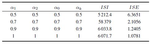
The fractional adaptive laws were implemented using the NID block of the Ninteger toolbox[13], developed for Matlab/Simulink. This implementation requires the definition of the number of poles and zeros of the transfer function ($N$) to be used in the approximation, as well as the frequency range where approximation is valid and where these poles/zeros lie. In general, large values of $N$ lead to more accurate approximation of the fractional order operator, and the converse is also true. In this paper the Crone approximation[14, 15, 16, 17, 18] of order 10 was used, with a frequency interval of $\left[0.01, 1, 000\right]$ rad/s. Table I shows the resulting values of ISI and ISE for these simulations.
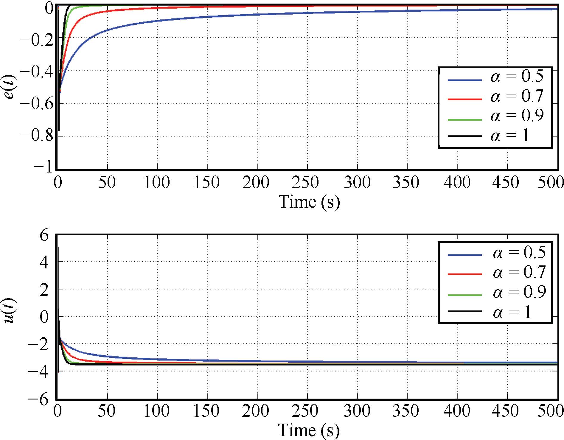
As can be seen from Table I, the lowest ISI value corresponds to the fractional case with lower order ($\alpha_1=\alpha_2=\alpha_0=\alpha_k=0.5$), increasing from there up to the integer order case. However, the behavior of the ISE is the opposite, being the case with the lowest ISI the one having the highest ISE.
Fig. 1shows the evolution of control error and the control signal for these simulations. As can be seen, the control signal is smoother for the fractional cases and also converges slowly to its final value, which explains why these cases have lower ISI. However, the convergence of the control error is slower for the fractional cases, which explains why they also have the higher ISE. Thus, there is a trade-off between the magnitudes of the ISI and ISE values, which must be analyzed before making a decision about what values to choose for the orders of the adaptive laws.

|
Download:
|
| Fig. 1 Control error $e\left(t\right)$ (above) and control signal $u\left(t\right)$ (below) for representative values of the orders in the adaptive laws, when the reference signal is a unit step. | |
How to choose the right orders in the adaptive laws is a question that always arises. The answer to this question, however, is not absolute, since it will depend on many factors. It can be seen in the very simple simulation example given here, where the same order was used for the four components of the adaptive laws, that different behaviors will be obtained depending on the selection.
For that reason, the first question we must answer is: how important is the ISI index with respect to the ISE index for our problem? As the reader may note, the answer to this question will strongly depend on the specific application. For example, for processes that are high energy consuming, a reduction of a 2% of the ISI could lead to million dollars savings in energy, and having probably a bit slower convergence speed of the control error.
Once this question is answered, it is still hard to choose the orders of the adaptive laws. Having in mind that there exists a trade-off between the ISI and the ISE, an optimization procedure appears to be the right option to decide.
In order to see how an optimization procedure can help to choose the orders $\alpha_1, \alpha_2, \alpha_0, \alpha_k$, we performed another simulation study. In this case, an optimization procedure was carried out using particle swarm optimization (PSO)[19], but other techniques could be used at designer will. The objective function used in this optimization process is presented in (17). Certainly, it includes both, the ISE and the ISI indexes, with their corresponding weighting factors to indicate how important is each index in the minimization problem.
| \begin{equation} J_{opt}=w_1\;ISE+w_2\;ISI. \label{eq:functional} \end{equation} | (17) |
For the optimization procedure we consider four cases. The first one takes into account only the ISE. The second, third and fourth take into account both, the ISE and the ISI, using different weighting factors $w_1, w_2$, as follows:
| \begin{equation} \begin{array}{l l l} {\rm Case}~1:\;\; w_1=1 & {\rm and} &w_2=0, \\ {\rm Case}~2:\;\; w_1=0.5& {\rm and} &w_2=0.5, \\ {\rm Case}~3:\;\; w_1=0.8& {\rm and} &w_2=0.2, \\ {\rm Case}~4:\;\; w_1=0.2& {\rm and} &w_2=0.8, \end{array} \label{eq:fact_peso} \end{equation} | (18) |
The optimization process delivers the best values of orders $\alpha_1, \alpha_2, \alpha_0$ and $\alpha_k$ minimizing the objective function $J_{opt}$ (17), using the weighting factors (18). The Matlab PSO toolbox[20] was used, with the most representative PSO parameters specified as:
1) Swarm size: 100
2) Number of iterations: 1 000
3) Initial inertia weight: 0.9
4) Final inertia weight: 0.4
The selection of these PSO parameters was made based on the works by []. The remaining PSO parameters were chosen at their default values.
For every case specified in (18), the optimization process was carried out ten times, obtaining ten sets of values for parameters $\alpha_1, \alpha_2, \alpha_0$ and $\alpha_k$. In order to select one set of parameters, a criterion function $J$ was calculated for each case, as it is specified in (19)
| \begin{equation} J=w_1\;ISE_{\rm norm}+w_2\;ISI_{\rm norm}, \label{eq:criterion} \end{equation} | (19) |
where $ISE_{\rm norm}$ and $ISI_{\rm norm}$ are the normalized values of $ISE$ and $ISI$ respectively. These normalized values were calculated as
| \begin{equation} ISE_{\rm norm}=\frac{ISE-ISE_{\min}}{ISE_{\max}-ISE_{\min}}, \label{eq:ISEnorm} \end{equation} | (20) |
and
| \begin{equation} ISI_{\rm norm}=\frac{ISI-ISI_{\min}}{ISI_{\max}-ISI_{\min}}, \label{eq:ISInorm} \end{equation} | (21) |
where $ISE_{\max}$, $ISE_{\min}$, $ISI_{\max}$ and $ISI_{\min}$ are the maximum and minimum values of $ISE$ and $ISI$, respectively, for the ten simulations.
The values of $ISI$ and $ISE$ were normalized because their absolute values were of very different magnitudes (see Table II), where the resulting orders are specified. Thus, normalization allows the resulting $ISI_{\rm norm}$ and $ISE_{\rm norm}$ to lie in the same interval $\left[0, 1\right]$, and then weighting them with weighting factors that are also in the interval $\left[0, 1\right]$ is much more fair.
|
|
Table Ⅱ RESULTING FRACTIONAL ORDERS FROM THE OPTIMIZATION PROCESS FOR THE UNSTABLE PLANT |
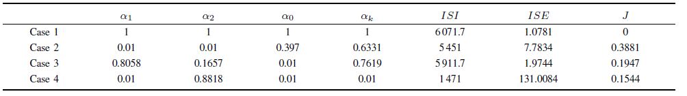
Analyzing the optimal set of parameters for the four cases, some conclusions can be drawn. It can be seen that the resulting optimal orders for Case 1 were all 1, that is, in this case the IOMRAC is the best solution. This means that when the control energy spent in the scheme is not taken into account, then the classic MRAC gives the best results.
However, for Case 2, Case 3 and Case 4, the resulting optimal orders are fractional. This means that, at least for this particular case analyzed, the recommended adaptive laws should not be the classic, if it is taken into account not only the behavior of the control error but also the energy used in the control. This empirical conclusion opens a lot of questions about MRAC, being a topic that deserves more research, from which interesting and useful results could be derived.
B. Numerical Results for the Marginally Stable PlantAs it was done in the case of the unstable plant, optimization process was carried out for the case of the marginally stable plant as well. All the details of the procedure used with the unstable plant were preserved, changing only the plant to be controlled. As a result of the optimization process, the fractional orders detailed in Table III were obtained. The values of the criterion function $J$ for these cases are also specified in Table III.
|
|
Table Ⅲ RESULTING FRACTIONAL ORDERS FROM THE OPTIMIZATION PROCESS FOR THE MARGINALLY STABLE PLANT |
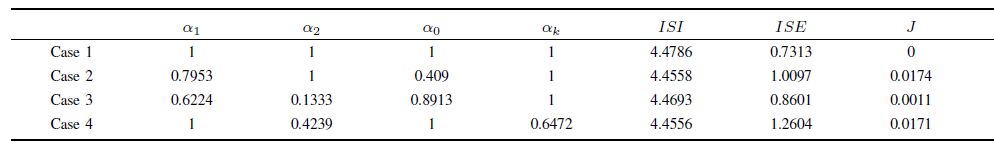
If we look at Table III, it can be noted that the resulting optimal orders for Case 1 were all 1. This is the same that happened for the unstable plant, that is, in this case the IOMRAC is the best solution. As we mentioned before, this means that when the control energy spent in the scheme is not taken into account, then the classic MRAC gives the best results.
As it was observed for the unstable plant, in this case it can be seen from Table III that for Case 2, Case 3 and Case 4, the resulting optimal orders are fractional or combinations of fractional and integer orders. Thus, when the energy used in the control scheme is taken into account, then the recommended adaptive laws should not be the integer order but fractional.
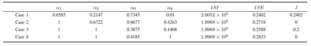
C. Numerical Results for the Stable PlantFinally, optimization process was carried out for the case of the stable plant. Again in this case, all the details of the procedure used with the unstable plant were preserved, changing only the plant to be controlled. As a result of the optimization process, the fractional orders and the values of $J$ obtained are detailed in Table IV.
|
|
Table Ⅳ RESULTING FRACTIONAL ORDERS FROM THE OPTIMIZATION PROCESS FOR THE STABLE PLANT |
As can be seen from Table IV, the main difference arising in the case of the stable plant is that the resulting optimal orders for Case 1 are not all 1, like in the case of unstable and marginally stable plant, but all fractional. The resulting optimal orders for Case 2, Case 3 and Case 4, are all fractional or combinations of fractional and integer orders, same as in the case of the two previously studied plants. Thus, although for the stable plant the optimal scheme for Case 1 is not the IOMRAC, the fractional orders do remain as the best options when the control energy spent in the scheme is taken into account.
Remark 1. Although the work presented here is preliminary, we must point out an important issue. Beside the orders of the adaptive laws ($\alpha_1$, $\alpha_2$, $\alpha_0$ and $\alpha_k$), MRAC schemes have some other design parameters such as adaptive gains $\gamma$ and initial conditions of the controller parameters. In this study, we used specific values for all these design parameters, and only the orders of the adaptive laws were varied. For that reason, a more complete study should include all these parameters in the decision making, being this a topic that is currently under investigation.
Ⅴ. CONCLUSIONSIn this paper, an empirical analysis of the control energy used in MRAC schemes has been presented, using orders for the adaptive laws in the interval $(0, 1]$. The analysis was made through simulation studies, including optimization procedures using PSO to select the orders of the adaptive laws. The behavior of the control energy spent by the system was analyzed through the integral of the squared control input ISI. The integral of the squared control error ISE was also included in the optimization process.
Simulation studies together with the optimization procedures were carried out for three different types of plants, and they have shown that, when the ISI is included in the objective function of the optimization to determine the orders of the adaptive laws, the resulting orders are fractional or combinations of fractional and integer orders. This is a very interesting result, since it suggests that the use of fractional adaptive laws could play an important role in the control energy management in MRAC schemes, which is an extremely important issue in today industry.
Since the results presented here are preliminary, research should be conducted to include other design parameters of the MRAC schemes into the optimization procedures.
| [1] | Narendra K S, Annaswamy A M. Stable Adaptive Systems. United States: Dover Publications Inc., 2005. |
| [2] | Kilbas A A, Srivastava H M, Trujillo J J. Theory and Applications of Fractional Differential Equations. New York: Elsevier, 2006. |
| [3] | Vinagre B M, Petráš I, Podlubny I, Chen Y Q. Using fractional order adjustment rules and fractional order reference models in model-reference adaptive control. Nonlinear Dynamics, 2002, 29(1-4): 269-279 |
| [4] | Ladaci S, Loiseau J, Charef A. Using fractional order filter in adaptive control of noisy plants. In: Proceedings of the 3rd International Conference on Advances in Mechanical Engineering and Mechanics. Hammamet, Tunisia, 2006. |
| [5] | Suárez J I, Vinagre B M, Chen Y Q. A fractional adaptation scheme for lateral control of an AGV. Journal of Vibration and Control, 2008, 14(9-10): 1499-1511 |
| [6] | Ma J, Yao Y, Liu D. Fractional order model reference adaptive control for a hydraulic driven flight motion simulator. In: Proceedings of the 41st Southeastern Symposium on System Theory. Tullahoma, TN: IEEE, 2009. 340-343 |
| [7] | He Y L, Gong R K. Application of fractional-order model reference adaptive control on industry boiler burning system. In: Proceedings of the 2010 International Conference on Intelligent Computation Technology and Automation (ICICTA). Changsha, China: IEEE, 2010. 750-753 |
| [8] | Sawai K, Takamatsu T, Ohmori H. Adaptive control law using fractional calculus systems. In: Proceedings of the 2012 SICE Annual Conference. Akita: IEEE, 2012. 1502-1505 |
| [9] | Aguila-Camacho N, Duarte-Mermoud M A. Fractional adaptive control for an automatic voltage regulator. ISA Transactions, 2013, 52(6): 807-815 |
| [10] | Ladaci S, Loiseau J J, Charef A. Fractional order adaptive high-gain controllers for a class of linear systems. Communications in Nonlinear Science and Numerical Simulation, 2008, 13(4): 707-714 |
| [11] | Charef A, Assabaa M, Ladaci S, Loiseau J J. Fractional order adaptive controller for stabilised systems via high-gain feedback. IET Control Theory and Applications, 2013, 7(6): 822-828 |
| [12] | Aguila-Camacho N, Duarte-Mermoud M A. Boundedness of the solutions for certain classes of fractional differential equations with application to adaptive systems. ISA Transactions, 2016, 60: 82-88 |
| [13] | Valério D, Da Costa J S. Ninteger: a non-integer control toolbox for Matlab. In: Proceedings of the 2004 Fractional Derivatives and Applications. Bordeaux, France: IFAC, 2004. |
| [14] | Oustaloup A. Systèmes Asservis Linéaires D'ordre Fractionnaire. Paris: Masson, 1983. |
| [15] | Oustaloup A. La Commande CRONE: Commande Robuste D'ordre Non Entier. Paris: Hermes, 1991. |
| [16] | Lanusse P. De la commande CRONE de première génération à la commande CRONE de troisième generation [Ph. D. dissertation], University of Bordeaux, France, 1994. |
| [17] | Oustaloup A. Non-Integer Derivation. Paris: Hermes, 1995. |
| [18] | Oustaloup A, Levron F, Mathieu B, Nanot F M. Frequency-band complex noninteger differentiator: characterization and synthesis. IEEE Transactions on Circuits and Systems I: Fundamental Theory and Applications, 2000, 47(1): 25-39 |
| [19] | Olsson A E. Particle Swarm Optimization: Theory, Techniques and Applications. New York: Nova Science Publishers, 2011. |
| [20] | Singh J. 03. The PSO toolbox. Tech. Rep.. Source Forge. Available: http://sourceforge.net/projects/psotoolbox, 2011. |
| [21] | Zamani M, Karimi-Ghartemani M, Sadati N, Parniani M. Design of a fractional order PID controller for an AVR using particle swarm optimization. Control Engineering Practice, 2009, 17(12): 1380-1387 |
| [22] | Chatterjee A, Mukherjee V, Ghoshal S P. Velocity relaxed and crazinessbased swarm optimized intelligent PID and PSS controlled AVR system. International Journal of Electrical Power & Energy Systems, 2009, 31(7-8): 323-333 |
| [23] | Ordóñez-Hurtado R H, Duarte-Mermoud M A. Finding common quadratic Lyapunov functions for switched linear systems using particle swarm optimisation. International Journal of Control, 2012, 85(1): 12-25 |