Ⅰ. Introduction

Fractional-order dynamic system has received a growing interest due to the fact that many real-world physical systems can be well characterized by fractional-order state equations and modeling various physical phenomena involves less parameters than traditional integer-order system ^[1]. Many useful analysis and synthesis results about fractional-order systems have emerged,such as stability ^{[2, 3, 4]} and Mittag-Leffler stability analysis ^[5],robust stability ^{[6, 7]},$H_\infty$ performance analysis ^[8],$H_\infty$ feedback control ^{[9, 10, 11]},and so on.

On the other hand,the Kalman-Yakubovich-Popov (KYP) Lemma has been proved to be a very strong tool to convert frequency domain inequalities (FDIs) to linear matrix inequalities (LMIs) ^[12]. Many control methods have been developed with the help of KYP Lemma ^{[13, 14, 15]}. However,KYP Lemma just only characterizes FDIs in entire frequency range and does not deal with the multiple FDIs in finite range. The generalized Kalman-Yakubovich-Popov (GKYP) Lemma provided in ^[16] extends the standard KYP Lemma to present the LMI characterization of FDIs in finite frequency range. It has been shown that the GKYP Lemma is profitable for system dissipative analysis and control synthesis problems which can be exactly converted to semidefinite programming or convex optimization problems. Based on GKYP Lemma,$H_\infty$ model reduction ^[17] and static output feedback control ^[18] problem for integer-order systems have been investigated over finite frequency. Furthermore,the $H_\infty$ performance analysis and $H_\infty$ control synthesis for fractional-order systems have been also considered in ^{[8, 9, 19, ]}. But these results are presented over the entire frequency range. It is worth noting that the $H_\infty$ synthesis problems over a finite frequency range is essentially different from the entire frequency range case this is because even the state feedback control problem cannot be completely solved via convex optimization ^[17].

In this paper,we will investigate the problem of $H_\infty$ static output feedback (SOF) controller synthesis for linear time-invariant fractional-order systems subject to finite frequency range. Based on the GKYP Lemma and a key projection lemma,necessary and sufficient condition is firstly established for the existence of a SOF controller that ensures the fractional order system is asymptotically stable and satisfies the prescribed $H_\infty$ performance index over a finite frequency range. Then,by using matrix congruence transformation,the feedback gain matrix is decoupled from matrix variables and parameterized by a scalar matrix. Moreover,two iterative algorithms are developed to solve this problem. Finally,numerical examples are given to demonstrate the effectiveness of our proposed method.

Notations. For a matrix $M$,its transpose and complex conjugate transpose are denoted by $M^{\rm T}$,$M^*$,respectively. The symbol $ H_n$ stands for the set of $n\times n$ Hermitian matrices. For a matrix $M\in {\bf H}_n$,inequalities $M>0$ $(\ge 0)$ and $M$ $<$ $0$ $(\le 0)$ denote positive (semi) definiteness and negative (semi) definiteness,respectively. For matrices $\Phi$ and $P$,$\Phi\otimes P$ means the Kronecker product. All the matrices are assumed to be of compatible dimensions and $\ast$ is used to denote the Hermitian part. For any matrix $M\in {\bf C}^{n\times n}$,${\rm Her}(X)=X$ $+$ $X^*$. ${\rm Re}(M)$ represents the real parts of the complex matrix $M$. For $G\in {\bf C}^{n\times m}$ and $\Pi\in {\bf H}_{n+m} $,a function $\sigma: {\bf C}^{n\times m}$ $\times$ ${\bf H}_{n+m}$ $\to$ ${\bf H}_{m}$ is defined by

\begin{eqnarray*} \sigma (G,\Pi):=\left[\begin{array}{l} G\\I_m\end{array}\right]^*\Pi\left[\begin{array}{l} G\\I_m\end{array}\right]. \end{eqnarray*}

${\rm j}$ denotes the imaginary unit.

Ⅱ. Preliminaries

In this paper, taking the physical meaning into consideration, the Caputo fractional-order derivative is used and defined as follows:

\begin{align*} D^{\alpha}f(t)=\frac{{\rm d}^{\alpha}f(t)}{{\rm d}t^{\alpha}}= \frac{1}{\Gamma(m-\alpha)}\int_{0}^{t}\frac{f^{(m)}(\tau)}{(t-\tau)^{\alpha+1-m}}{\rm d}\tau, \end{align*}

where $f(t)$ is a time-dependent function,$\alpha$ represents the order of the derivative ($m - 1 \le \alpha < m$, $m$ is an integer).

Consider the following linear time-invariant fractional-order system admitting a pseudo state space representation of the form

\begin{align}\label{system model} \begin{cases} D^{\alpha}x(t)=Ax(t)+B_{1}u(t)+Bw(t),\\[1mm] z(t)=C x(t)+Dw(t),\\[1mm] y(t)=C_{y}x(t), \end{cases} \end{align}

(1)

where $\alpha$ is the fractional order and $\alpha\in (0,\ 2)$. $x(t)\in {\bf R}^{n}$ is system state,$u(t)\in {\bf R}^m$ is control input,$w(t)\in {\bf R}^{q}$ is disturbance input,$z(t)\in {\bf R}^{s}$ is control output,$y(t)\in{\bf R}^l$ is measured output. $A\in {\bf R}^{n\times n}$,$B_1\in {\bf R}^{n\times m}$, $B\in {\bf R}^{n\times q}$,$C$ $\in$ ${\bf R}^{s\times n}$,$C_y\in {\bf R}^{l\times n}$,and $D \in {\bf R}^{s\times q}$ are known matrices.

In general,the frequency ranges can be visualized as the following set of complex numbers that represents certain curves on the complex plane:

\begin{eqnarray}\label{cv} \Lambda(\Phi,\Psi):=\{\lambda\in {\bf C}| \sigma(\lambda,\Phi)=0,\sigma(\lambda,\Psi)\geq 0\}, \end{eqnarray}

(2)

where $\Phi$,$\Psi\in{\bf H}_2$.

Define $\bar{\Lambda}(\Phi,\Psi)=\Lambda(\Phi,\Psi)\cup\{ \infty\}$ if $\Lambda$ is bounded,otherwise $\bar{\Lambda}(\Phi,\Psi)=\Lambda(\Phi,\Psi)$.

By choosing appropriate $\Phi$ and $\Psi$ in (2),the set $\Lambda(\Phi,\Psi)$ can be specified to define a certain range of the frequency curve. For fractional-order system,we can choose

$$\Phi=\left[\begin{array}{cc} 0 & r\\ \ast & 0\end{array}\right] $$

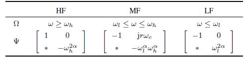
to represent the curve $\Lambda=\{ ({\rm j}\omega)^\alpha| \omega\in \Omega\}$,where $r={\rm e}^{{\rm j}\theta}$,$\theta$ $=$ $(\alpha-1)\pi/2$,$\Omega$ is a subset of real numbers specified by appropriate choice of $\Psi$,Table Ⅰ shows an example.

In Table Ⅰ,$\omega_c:=({\omega_l^\alpha+\omega_h^\alpha})/{2}$, $\omega_h\geq 0$,$\omega_l\geq 0$,and HF,MF and LF denote high, middle and low frequency ranges,respectively.

In this paper,we focus on the static output feedback controller in the following form:

\begin{align} u(t)=Ky(t), \end{align}

(3)

then,we have the following closed-loop system

\begin{align} \begin{cases} D^{\alpha}x(t)=\hat{A}x(t)+B\omega(t),\\[1mm] z(t)=C x(t)+D\omega(t), \end{cases} \end{align}

(4)

where $\hat{A}=A+B_{1}KC_{y}$.

Therefore,the finite frequency $H_{\infty}$ static output feedback control problem can be formulated as follows.

Problem FF-${\pmb H_{\pmb\infty}}$-SOFC (Finite frequency ${\pmb H}_{\pmb\infty}$ static output feedback control) For a pre-specified frequency range $\Lambda(\Phi,\Psi)$ and a given performance index $\gamma>0$,The problem of the $H_{\infty}$ static output feedback control over frequency range $\Lambda(\Phi,\Psi)$ is to find a static output feedback controller (2) such that:

1) The closed-loop system (3) is asymptotically stable.

2) The transfer function $G(s)$ of closed-loop system (3) satisfies the finite frequency $H_{\infty}$ performance ${\rm sup}_{\omega\in\Lambda(\Phi,\Psi)}\bar\sigma(G({\rm j}\omega))< \gamma$,where $G(s)=C(s^\alpha I- \hat A)^{-1}B+D$,$\bar\sigma$ denotes the maximum singular value of a matrix.

The following lemma is very useful in the proofs of the main results of this paper.

Lemma 1 ^[11] Let $A\in {\bf R}^{n\times n}$,the linear time-invariant system $D^{\alpha}x(t)=Ax(t)$ with $\alpha\in(0, 1)$ is asymptotically stable if and only if there exists Hermitian matrix $H>0$ such that $({\rm Re}(rH))^{\rm T}A^{\rm T}+A({\rm Re}(rH))<0$.

Lemma 2 ^[11] Let $A\in {\bf R}^{n\times n}$,the linear time-invariant system $D^{\alpha}x(t)=Ax(t)$ with $\alpha\in(1, 2)$ is asymptotically stable if and only if there exists Hermitian matrix $H>0$ such that $rHA^{\rm T}+\bar{r}AH<0$.

Lemma 3~(GKYP Lemma) ^{[16, 19]} Given real matrices $A$, $B$,$C$,$D$,a real symmetric matrix $\Pi$,and $\Phi$,$\Psi$, $\in {\bf H}_2$,let $G(\lambda)=C(\lambda I-A)^{-1}B+D$. Then the frequency range inequality

\begin{eqnarray*} \left[\begin{array}{c} G(\lambda)\\ I\end{array}\right]^*\Pi \left[\begin{array}{c} G(\lambda)\\ I\end{array}\right]<0 \end{eqnarray*}

holds for all $\lambda\in \bar{\Lambda}(\Phi,\Psi)$ if and only if there exist Hermitian matrices $P$ and $Q>0$ such that

\begin{align*} &\left[\begin{array}{cc} A & I\\C & 0\end{array}\right](\Phi \otimes P+\Psi \otimes Q)\left[\begin{array}{cc} A & I\\C & 0\end{array}\right]^{\rm T}\\&\qquad +\left[\begin{array}{cc} B& 0\\D & I\end{array}\right]\Pi\left[\begin{array}{cc} B& 0\\D & I\end{array}\right]^{\rm T}<0. \end{align*}

Remark 1. Let

$$\Pi= \left[ \begin{array}{cc} I & 0 \\ 0 & \gamma^2 I \end{array} \right] $$

or

$$\Pi= \left[ \begin{array}{cc} 0 & -I \\ -I & 0 \end{array} \right], $$

the characterization of Lemma 3 turns into the bounded real lemma and positive real lemma.

Lemma 4~ (Projection Lemma) ^[20] Given a symmetric matrix $\Xi\in {\bf R}^{m\times m}$ and two matrices $P$,$Q$ of column dimension $m$,consider the problem of finding some matrix $\Theta$ of compatible dimensions such that

\begin{eqnarray}\label{Projection LMI} \Xi+P^{\rm T}\Theta^{\rm T}Q+Q^{\rm T}\Theta P<0. \end{eqnarray}

(5)

Denote by $ \aleph_P$,$ \aleph_Q$ any matrices whose columns form basis of the null space of $P$ and $Q$,respectively. Then (5) is solvable for $\Theta$ if and only if

\begin{align*} \begin{cases} \aleph^{\rm T}_P\Xi \aleph_P < 0,\\[1mm] \aleph^{\rm T}_Q\Xi \aleph_Q <0.\end{cases} \end{align*}

Ⅲ. Main results

In this section,we will firstly investigate the $H_{\infty}$ static output feedback control for fractional-order systems over middle frequency ranges. Based on the GKYP Lemma and the projection lemma,we will give the necessary and sufficient condition that the problem of FF-$H_{\infty}$-SOFC is solvable.

Theorem 1. Given performance index $\gamma>0$,fractional order $\alpha\in(0,1)$,system matrices $A,B_{1},B,C,D,C_{y}$,a feedback gain $K$ and finite frequency range $\Lambda_{MF}=\{\omega\in {\bf R}:$ $\omega_{l}$ $\leq$ $\omega$ $\leq$ $\omega_{h}$,$\omega_{l},\omega_{h}\geq0\}.$ Problem FF-$H_{\infty}$-SOFC is solvable if and only if there exist Hermitian matrices $H>0$,$Q>0$,$P$,and real matrix $E=[E_{1},\ E_{2}]$ such that the following matrix inequalities hold:

\begin{eqnarray}\label{LMI1} \Xi={\rm Her}({ \hat{A}({\rm Re}(rH))})<0, \end{eqnarray}

(6)

and

\begin{eqnarray}\label{LMI2} \Sigma=\left[ \begin{array}{cccc} -Q & \Sigma_{12} &-E_{2} &0 \\ \ast & \Sigma_{22} & \Sigma_{23} & B \\ \ast & \ast & \Sigma_{33} & D\\ \ast & \ast & \ast & -I\\ \end{array} \right]<0, \end{eqnarray}

(7)

where $r={\rm e}^{{\rm j}\theta}$,$\theta=(\alpha-1)\pi/2$,$ \hat{A}=A+B_{1}KC_{y},$ and

$$\eqalign{ & {\Sigma _{12}} = rP + {\rm{j}}r{\omega _c}Q - {E_1}, \cr & {\Sigma _{22}} = - \omega _l^\alpha \omega _h^\alpha Q + {\rm{Her}}(\hat A{E_1}), \cr & {\Sigma _{23}} = \hat A{E_2} + E_1^{\rm{T}}{C^{\rm{T}}}, \cr & {\Sigma _{33}} = - {\gamma ^2}I + {\rm{Her}}(C{E_2}). \cr} $$

Proof. (Necessity). It follows from Lemma 1 and Lemma 3 that the problem of FF-$H_{\infty}$-SOFC is solvable if and only if there exist Hermitian matrices $H>0$,$Q>0$ and $P$ such that the following matrix inequalities hold. That is,

\begin{eqnarray*} \Xi={\rm Her}({ \hat{A}({\rm Re}(rH))})<0, \end{eqnarray*}

and

\begin{align*} &\left[ \begin{array}{cc} \hat{A} & I \\ C & 0 \\ \end{array} \right]\left[ \begin{array}{cc} -Q & r P+{\rm j}r\omega_{c}Q \\ \bar{r}P-{\rm j}\omega_{c}Q & -\omega_{l}^\alpha\omega_{h}^\alpha Q \\ \end{array} \right]\left[ \begin{array}{cc} \hat{A} & I \\ C & 0 \\ \end{array} \right]^{\rm T}\\[1mm] &\qquad +\left[ \begin{array}{cc} B & 0 \\ D & I \\ \end{array} \right]\left[ \begin{array}{cc} I & 0 \\ 0 & -\gamma^{2}I \\ \end{array} \right]\left[ \begin{array}{cc} B & 0 \\ D & I \\ \end{array} \right]^{\rm T}\\[1mm] &\qquad =\left[ \begin{array}{ccc} \hat{A} & I & 0 \\ C & 0 & I \\ \end{array} \right]\Theta\left[ \begin{array}{ccc} \hat{A} & I & 0 \\ C & 0 & I \\ \end{array} \right]^{\rm T}<0, \end{align*}

where

\begin{eqnarray*} \Theta=\left[ \begin{array}{ccc} -Q & r P+{\rm j}r\omega_{c}Q & 0 \\ \ast & -\omega_{l}^\alpha\omega_{h}^\alpha Q+BB^{\rm T} & BD^{\rm T} \\ \ast & \ast & DD^{\rm T}-\gamma^{2}I \\ \end{array} \right]. \end{eqnarray*}

Note that

\begin{eqnarray*} \left[ \begin{array}{ccc} I & 0 & 0 \\ \end{array} \right]\Theta\left[ \begin{array}{ccc} I & 0 & 0 \\ \end{array} \right]^{\rm T}=-Q<0, \end{eqnarray*}

and denote that

\begin{eqnarray*} \Gamma=\left[ \begin{array}{ccc} -I & \hat{A}^{\rm T} & C^{\rm T} \\ \end{array} \right],\ \ \Lambda= \left[ \begin{array}{ccc} 0 & I & 0 \\ 0 & 0 & I \\ \end{array} \right], \end{eqnarray*}

then, we can obtain

\begin{eqnarray*} \aleph_{\Gamma}=\left[ \begin{array}{cc} \hat{A}^{\rm T} & C \\ I & 0 \\ 0 & I \\ \end{array} \right],\ \ \aleph_{\Lambda}=\left[ \begin{array}{ccc} I & 0 & 0 \\ \end{array} \right]^{\rm T}, \end{eqnarray*}

and

\begin{eqnarray*} \aleph_{\Gamma}^{\rm T}\Theta\aleph_{\Gamma}<0,\ \ \aleph_{\Lambda}^{\rm T}\Theta\aleph_{\Lambda}<0. \end{eqnarray*}

It follows from the projection lemma that there exists a real matrix $E=[E_1\ E_2]$ such that

\begin{eqnarray*} \Theta+\Gamma^{\rm T}E\Lambda+\Lambda^{\rm T}E^{\rm T}\Gamma<0, \end{eqnarray*}

which implies $\Sigma<0$ holds by Schur complement lemma.

(Sufficiency). It follows from Schur complement lemma that $\Xi_2<0$ is equivalent to $\Theta+\Gamma^{\rm T}E\Lambda+\Lambda^{\rm T}E^{\rm T}\Gamma<0$. Using the projection lemma,$\aleph_{\Gamma}^{\rm T}\Theta\aleph_{\Gamma}<0$ holds. Therefore, the sufficiency is trivially true.

Remark 2. In the above theorem,the feedback gain $K$ is coupled with matrix variables and is intrinsically non convex. In the following theorem,the feedback gain matrix $K$ will be decoupled from matrices $H$,$E_{1}$,and $E_{2} $, simultaneously,and will be parameterized by a positive scalar matrix.

Theorem 2. Given performance index $\gamma>0$,fractional order $\alpha\in(0,1)$,system matrices $A$,$B_{1}$,$B$,$C$,$D$ and $C_{y},$ and the finite frequency range $\Lambda_{MF}=\{\omega\in {\bf R}:\omega_{l}\leq\omega\leq$ $\omega_{h}$,$\omega_{l},\omega_{h}\geq0\}.$ Problem FF-$H_{\infty}$-SOFC is solvable if and only if there exist Hermitian matrices $H>0$,$Q>0$,$P$,real matrices $E=[E_{1},\ E_{2}]$,$U$,and a scalar $\epsilon>0$,such that the following matrix inequalities hold

\begin{eqnarray}\label{LMI3} \bar{\Xi}=\left[ \begin{array}{cc} \bar{\Xi}_{11} & -({\rm Re}(rH))^{\rm T}-B_{1}LC_{y} \\ \ast & -\epsilon I \\ \end{array} \right]<0, \end{eqnarray}

(8)

and

\begin{eqnarray}\label{LMI4} \bar{\Sigma}= \left[ \begin{array}{ccccc} -Q & \bar{\Sigma}_{12} & -E_{2} & 0 & 0 \\ \ast & \bar{\Sigma}_{22}& \bar{\Sigma}_{23} & B & \bar{\Sigma}_{25} \\ \ast & \ast & \bar{\Sigma}_{33} & D & -E_{2}^{\rm T} \\ \ast & \ast & \ast & -I & 0 \\ \ast & \ast & \ast & \ast & -\epsilon I \\ \end{array} \right]<0, \end{eqnarray}

(9)

where $r={\rm e}^{{\rm j}\theta}$,$\theta=(\alpha-1)\pi/2$, and

\begin{align*} \bar{\Xi}_{11}=&\ {\rm Her}\left( A({\rm Re}(rH))-B_1LC_{y}U^{\rm T}B_1^{\rm T}\right)\\ &\,+\epsilon B_1UU^{\rm T}B_1^{\rm T},\\[1mm] \bar{\Sigma}_{12}=&\ rP+{\rm j}r\omega_{c}Q-E_{1},\\[1mm] \bar{\Sigma}_{22}=&\,-\omega_{l}^\alpha\omega_{h}^\alpha Q+{\rm Her}(AE_1-B_1LC_{y}U^{\rm T}B_1^{\rm T})\\ &\,+\epsilon B_1UU^{\rm T}B_1^{\rm T},\\[1mm] \bar{\Sigma}_{23}=&\ AE_{2}+E_{1}^{\rm T}C^{\rm T},\\[1mm] \bar{\Sigma}_{33}=&\,-\gamma^{2}I+{\rm Her}(CE_{2}),\\[1mm] \bar{\Sigma}_{25}=&\,-E_{1}^{\rm T}-B_1LC_{y}. \end{align*}

Moreover,the static output feedback control gain is designed as $K=\epsilon^{-1} L$.

Proof. (Necessity). It follows from Theorem 1 that problem FF-$H_{\infty}$-SOFC is solvable if and only if there exist Hermitian matrices $H>0$,$Q>0$,$P$ and real matrix $E=[E_{1},E_{2}]$ such that (6) and (7) hold. It is always possible to find a sufficiently large scalar $\epsilon$ such that

\begin{eqnarray*} \left[ \begin{array}{cc} {\rm Her}(\hat{A}({\rm Re}(rH))) &-{\rm Re}(rH)^{\rm T} \\ \ast & -\epsilon I \\ \end{array} \right]<0,\,\ \end{eqnarray*}

and

\begin{eqnarray*} \left[ \begin{array}{cc} \Xi_2 & \Upsilon^{\rm T}\\ \ast & -\epsilon I \\ \end{array} \right]<0, \end{eqnarray*}

where $\Upsilon=[0\ -E_{1}\ -E_{2}\ \ 0]$.

Taking congruence transformation yields

\begin{align}\label{tilder xi1} & \Gamma_{1}^{\rm T}\ \left[ \begin{array}{cc} {\rm Her}(\hat{A}({\rm Re}(rH))) & -({\rm Re}(rH) )^{\rm T} \\ \ast & -\epsilon I \\ \end{array} \right]\Gamma_{1}\nonumber\\[1mm] &\qquad = \left[ \begin{array}{cc} \Phi_{11} &\Phi_{12} \\ \ast & -\epsilon I \\ \end{array} \right]<0. \end{align}

(10)

with

\begin{align*} &\Gamma_{1}=\left[ \begin{array}{cc} I & 0 \\ (B_{1}KC_{y} )^{\rm T}& I \\ \end{array} \right],\\[1mm] & \Phi_{11}={\rm Her}( A({\rm Re}(rH))-\epsilon (B_{1}KC_{y})(B_{1}KC_{y})^{\rm T},\\[1mm] & \Phi_{12}=-({\rm Re}(rH))^{\rm T}-\epsilon B_{1}KC_{y}. \end{align*}

Let $\epsilon K=L$ and note that

$$B_1(LC_{y}-\epsilon U)\epsilon^{-1}(LC_{y}-\epsilon U)^{\rm T}B_1^{\rm T}\geq0$$

holds for any real matrix $U$. Expanding this inequality,one has

\begin{align}\label{add ineq} &-(B_1LC_{y})\epsilon^{-1}(B_1LC_{y})^{\rm T}\nonumber\\[1mm] &\qquad \leq-B_1LC _{y}U ^{\rm T}B_1^{\rm T}-B_1U(LC_{y})^{\rm T}B_1^{\rm T}+\epsilon B_1UU^{\rm T}B_1^{\rm T}. \end{align}

(11)

Using above inequality and combining (10),we get (8). In the same way,taking congruence transformation, we have

$$\Gamma_{2}^{\rm T}\left[ \begin{array}{cc} \Xi_2 & \Upsilon^{\rm T} \\ \ast & -\epsilon I \\ \end{array} \right]\Gamma_{2}<0,$$

with

$$ \Gamma_{2}=\left[ \begin{array}{ccccc} I & 0 & 0 & 0 & 0 \\ 0 & I & 0 & 0 & 0 \\ 0 & 0 & I & 0 & 0 \\ 0 & 0 & 0 & I & 0 \\ 0 & (B_{1}KC_{y})^{\rm T} & 0 & 0 & I \\ \end{array} \right].$$

Let $\epsilon K=L$ and use inequality (11),we get (9).

(Sufficiency). Suppose that there exist Hermitian matrices $H>0$, $Q>0$,$P$,real matrices $E=[E_{1},\ \ E_{2}]$,$U$ and a scalar $\epsilon>0$ such that (8) and (9) hold. From (11), (8) implies that

\begin{eqnarray*} \left[ \begin{array}{cc} \tilde{\Phi}_{11} & - ({\rm Re}(rH))^{\rm T}-B_{1}LC_{y}\\ \ast & -\epsilon I \\ \end{array} \right]<0, \end{eqnarray*}

where

$$\tilde{\Phi}_{11}={\rm Her}( A({\rm Re}(rH))-(B_1LC_{y})\epsilon ^{-1}(LC_{y})^{\rm T}B_1^{\rm T},$$

choosing $U=\epsilon ^{-1}LC_{y}$ yields

\begin{eqnarray*} \left[ \begin{array}{cc} \bar{\Phi}_{11} & -({\rm Re}(rH))^{\rm T}-\epsilon B_{1}U\\ \ast & -\epsilon I \\ \end{array} \right]<0, \end{eqnarray*}

where,$\bar{\Phi}_{11}={\rm Her}( A({\rm Re}(rH))-\epsilon B_1UU^{\rm T}B_1^{\rm T} $.

Therefore,using congruence transformation and letting $\epsilon^{-1}L$ $=$ $K$,we can conclude that

\begin{eqnarray*} \left[ \begin{array}{cc} {\rm Her}(\hat{A}({\rm Re}(rH))) &-({\rm Re}(rH))^{\rm T} \\ \ast & -\epsilon I \\ \end{array} \right]<0, \end{eqnarray*}

and $ {\rm Her}(\hat{A}({\rm Re}(rH))) <0$. Similarly,one can deduce that (9) implies (7).

Remark 3. Based on congruence transformation,the feedback gain $K$ can be decoupled from $H$,$E_{1}$ and $E_{2}$ simultaneously, and parameterized by a positive scalar $\epsilon$. Note that the matrix inequalities in (8) and (9) are still bilinear, however,we can fix $U$ to make them linear. Using the method provided in ^{[21, 22]},we defined $\eta\in {\bf R}$ satisfying that

\begin{align*} \begin{cases} \bar{\Xi}-{\rm diag}\{\eta I,0\}<0,\\[1mm] \bar{\Sigma}-{\rm diag}\{0,\eta I,0,0,0\}<0.\\ \end{cases} \end{align*}

It is easily known from the proof of Theorem 1 that $\eta$ achieves its minimum when $U=\epsilon^{-1}LC_{y}$,which naturally leads to an iterative LMI (ILMI) algorithm.

Algorithm 1 (ILMI algorithm).

Step 1. Set $j=1$. For a given $H_{\infty}$ performance level $\gamma>0$,and the finite frequency range $\Lambda_{FF}=\{\omega\in {\bf R}:\omega_{l}\leq\omega\leq$ $\omega_{h}$,$\omega_{l}, \omega_{h}\geq0\}$. Solve the following relaxed LMIs

\begin{eqnarray}\label{LMI5} {\rm Her}(A({\rm Re}(rH))+B_{1}W_{1})<0, \end{eqnarray}

(12)

and

\begin{eqnarray}\label{LMI6} \left[ \begin{array}{cccc} -Q & \hat{\Phi}_{12} & -E_{2} & 0 \\ \ast & \hat{\Phi}_{22} & \hat{\Phi}_{23} & B \\ \ast &\ast & \hat{\Phi}_{33} & D \\ \ast &\ast &\ast & -I \\ \end{array} \right]<0. \end{eqnarray}

(13)

where

\begin{align*} \hat{\Phi}_{12}&=r P+{\rm j}r\omega_{c}Q-E_{1},\\[1mm] \hat{\Phi}_{22}&=-\omega_{l}^\alpha\omega_{h}^\alpha Q+{\rm Her}(AE_{1}+B_{1}W_{2}),\\[1mm] \hat{\Phi}_{23}&=AE_{2}+B_{1}W_{3}+E_{1}^{\rm T}C^{\rm T},\\[1mm] \hat{\Phi}_{33}&=-\gamma^{2}I+Her(CE_{2}), \end{align*}

with variables in $S\triangleq \{$Hermitian matrices $H>0$,$Q>0$,$P$,and real matrices,$E_{1}$,$E_{2}$,$W_{1}$,$W_{2}$ and $W_{3}\}.$

The initial value $U_{1}$ is obtained as

$$U_{1}=W_{1}({\rm Re}(rH))^{-1}.$$

Step 2. For fixed $U_{j}$,solve the following minimization problem for matrix variables in the set $S\triangleq\{$Hermitian matrices $H>0$,$Q>0$,$P,$ real matrices $E=[E_{1},E_{2}]$,$U$ and a scalar $\epsilon>0\}$

\begin{align}\label{optimization LMI} &\min\ \eta,\nonumber\\[2mm] &\,{\rm s.t.} \begin{cases} \bar{\Xi}-{\rm diag}\{\eta I,0\}<0,\\ \bar{\Sigma}-{\rm diag}\{0,\eta I,0,0,0\}<0,\\ \end{cases} \end{align}

(14)

where $\bar{\Xi}$ and $\bar{\Sigma}$ are defined in (8) and (9) respectively. Denote the obtained $\eta$ as $\eta_{j}$.

Step 3. If $\eta_{j}<0,$ then a desired feedback gain is obtained as $K=\epsilon^{-1} L$.

Step 4. Fix $\eta=\eta_{j}$,minimize $\epsilon$ such that LMIs (14) hold,denote the obtained $\epsilon$ and $L$ as $\epsilon_{j}$ and $L_{j}$.

Step 5. If $|\eta_{j}-\eta_{j-1}|/\eta_{j-1}<\tau$,where $\tau$ is a prescribed tolerance,then this algorithm fails to find the desired feedback gain $K$,stop; If not,update $\eta_{j+1}$ as $U_{j+1}=\epsilon_{j}^{-1}L_{j}C_{y}$. Set $j$ $:=$ $j$ $+$ $1$ and go to Step 2.

Before employing the ILMI algorithm, it is suggested to find some initial value which is ``close'' to the desired solution. We adopt the following initial optimization algorithm provided in ^[11]. Denote $\bar{W}=[W_{1},\ W_{2},\ W_{3}]$ and $\bar{E}=[{\rm Re}(rH),\ E_{1} ,\ E_{2}]$.

Algorithm 2 (Initial optimisation).

Step 1. Set $j=1$. For a given $H_{\infty}$ performance level $\gamma>0$,and the finite frequency range $\Lambda_{FF}=\{\omega\in {\bf R}:\omega_{l}\leq\omega\leq\omega_{h},$ $\omega_{l}, \omega_{h}\geq0\},$ find Hermitian matrices $H>0$,$Q>0$,$P$, and real matrices $W_{1}$,$W_{2}$,$W_{3}$ such that LMIs (12}) and (13) hold. Denote the feasible solution $\bar{E}$ and $\bar{W}$ as $\bar{E_{j}}$ and $\bar{W_{j}}.$

Step 2. Fix $\bar{E}=\bar{E_{j}}$,minimize $\delta=\|\bar{W}- N\otimes \bar{E}\|_{2},$ such that LMIs (12) and (13) hold,where $N$ is a real matrix variable. Denote the obtained $N$ as $N_{j}$.

Step 3. Fix $N=N_{j}$,minimize $\delta=\|\bar{W}-N \otimes \bar{H}\|_{2},$ such that LMIs (13) and (12) hold. Denote the minimized $\delta$ as $\delta_{j}$.

Step 4. Set $j:=j+1$,and repeat { Step 2} and { Step 3}. If $|\delta_{j}-\delta_{j-1}|/ \delta_{j-1}\leq \mu$,where $\mu$ is a prescribed tolerance,then stop. The initial value $U_{1}$ is given by $U_{1}=W_{1}({\rm Re}(rH))^{-1}$.

Follow the similar line,we can give the condition that the problem of FF-$H_{\infty}$-SOFC is solvable over low frequency range as follows.

Theorem 3. Given performance index $\gamma>0$,fractional order $\alpha\in(0,1)$,system matrices $A$,$B_{1}$,$B$,$C$, $D$,$C_{y}$,a feedback gain $K$ and finite frequency range $\Lambda_{LF}=\{\omega\in$ ${\bf R}:$ $\omega\leq\omega_{l}$, $\omega_{l}\geq0\}$. Problem FF-$H_{\infty}$-SOFC is solvable if and only if there exist Hermitian matrices $H>0$,$P$ and $Q$ $>$ $0$, real matrix $U$,$E=[E_{1},\ E_{2}]$ and real scalar $\epsilon$ such that the following matrix inequalities hold

\begin{eqnarray*} \tilde{\Xi}=\left[ \begin{array}{cc} \tilde{\Xi}_{11} & -({\rm Re}(rH))^{\rm T}-B_{1}LC_{y} \\ \ast & -\epsilon I \\ \end{array} \right]<0, \end{eqnarray*}

and

\begin{eqnarray*} \tilde{\Sigma}=\left[\begin{array}{ccccc} -Q & rP-E_{1} & -E_{2} & 0 & 0\\ \ast & \tilde{\Sigma}_{22} & \tilde{\Sigma}_{23} & B & \tilde{\Sigma}_{25}\\ \ast & \ast & \tilde{\Sigma}_{33} & D & -E_{2}^{\rm T}\\ \ast & \ast & \ast & -I & 0\\ \ast & \ast & \ast & \ast & \epsilon I \end{array}\right]<0, \end{eqnarray*}

where $r={\rm e}^{{\rm j}\theta}$,$\theta=(\alpha-1)\pi/2$,and

\begin{align*} \tilde{\Xi}_{11}=&\ {\rm Her}\left( A({\rm Re}(rH))-B_1LC_{y}U^{\rm T}B_1^{\rm T}\right)\\ &\,+\epsilon B_1UU^{\rm T}B_1^{\rm T},\\[1mm] \tilde{\Sigma}_{23}=&\ AE_{2}+E_{1}^{\rm T}C^{\rm T},\\[1mm] \tilde{\Sigma}_{22}=&\ \omega_{l}^{2\alpha}Q+{\rm Her}(AE_{1}-B_{1}LC_{y}U^{\rm T}B_{1}^{\rm T})\\ &\,+\epsilon B_{1}UU^{\rm T}B_{1}^{\rm T},\\[1mm] \tilde{\Sigma}_{25}=&\,-E_{1}^{\rm T}-B_{1}LC_{y},\\[1mm] \tilde{\Sigma}_{33}=&\,-\gamma^{2}I+{\rm Her}(CE_{2}). \end{align*}

Moreover,the static output feedback control gain is designed as $K=\epsilon^{-1} L$.

For highest frequency case,we can refer to the designed method in ^[17] and use the following condition.

Theorem 4. Given performance index $\gamma>0$,fractional order $\alpha\in(0,1)$,system matrices $A$,$B_{1}$,$B$,$C$,$D$ and $C_{y}$,and the finite frequency range $\Lambda_{HF}=\{\omega\in {\bf R}:\omega\geq\omega_{h},\omega_{h}\geq0\}$. Problem FF-$H_{\infty}$-SOFC is solvable if and only if there exist Hermitian matrices $H>0$,$P$,and $Q>0$,real matrix $U$,and a scalar $\epsilon>0$,such that the following matrix inequalities hold

\begin{eqnarray*} \hat{\Xi}=\left[ \begin{array}{cc} \hat{\Xi}_{11} & -({\rm Re}(rH))^{\rm T}-B_{1}LC_{y} \\ \ast & -\epsilon I \\ \end{array} \right]<0, \end{eqnarray*}

and

\begin{eqnarray*} \hat{\Sigma}=\left[\begin{array}{ccccc} \hat{\Sigma}_{11} & \bar{r}PC^{\rm T} & AQ & B & P+rB_{1}LC_{y}\\ \ast & -\gamma^{2}I & CQ & D & 0\\ \ast & \ast & -Q & 0 & rQ\\ \ast & \ast & \ast & -I & 0\\ \ast & \ast & \ast & \ast & -\epsilon I \end{array}\right]<0, \end{eqnarray*}

where $r={\rm e}^{{\rm j}\theta}$,$\theta=(\alpha-1)\pi/2$,and

\begin{align*} \hat{\Xi}_{11}=&\ {\rm Her}\left( A({\rm Re}(rH))-B_1LC_{y}U^{\rm T}B_1^{\rm T}\right)\\ &\,+\epsilon B_1UU^{\rm T}B_1^{\rm T},\\[1mm] \hat{\Sigma}_{11}=&\ {\rm Her}(rAP-B_{1}LC_{y}U^{\rm T}B_{1}^{\rm T})-\omega_{h}^{2\alpha}Q\\ &\,+\epsilon B_{1}UU^{\rm T}B_{1}^{\rm T}. \end{align*}

Moreover,the static output feedback control gain is designed as $K=\epsilon^{-1} L$.

Remark 4. The designed algorithms of $H_\infty$ static output feedback controller for fractional order system over high frequency and low frequency ranges can refer to the middle frequency case and hence is omitted for brevity.

Remark 5. When the problem of FF-$H_{\infty}$-SOFC for system with the fractional order $\alpha\in[1,2)$ case is considered,we just need to replace the stability condition based on Lemma 2. For example,we just replace LMI (8) by

\begin{eqnarray*} \left[ \begin{array}{cc} \Psi_{11} & -H-\bar{r}B_{1}LC_{y} \\ \ast & -\epsilon I \\ \end{array} \right]<0, \end{eqnarray*}

where $\Psi_{11}={\rm Her}\left( \bar{r}AH-B_1LC_{y}U^{\rm T}B_1^{\rm T}\right)+\epsilon B_1UU^{\rm T}B_1^{\rm T}.$

Ⅳ. Numerical Example

Example 1. Consider the system (1) with the following parameters:

\begin{align*} &A=\left[\begin{array}{cc} -8 & -0.8\\-2 & 0.5\end{array}\right],~~ B_1=\left[ \begin{array}{c} -0.6\\ 2 \end{array} \right],~~B=\left[ \begin{array}{c} 1\\ 0.1 \end{array} \right],\\[1mm] & C=\left[ \begin{array}{cc} 1.2&2 \end{array} \right],~~C_y=\left[ \begin{array}{cc} 1&-130 \end{array} \right],~~ D=0.1, \\[1mm] & \alpha=0.8,~~\omega_l=0.2,~~ \omega_h=4. \end{align*}

The eigenvalues of $A$ are $\lambda_1=-8.1842$,$\lambda_2=0.6842$, which implies the open-loop system is unstable. Using Algorithm 2, the initial value $U_1$ is obtained as

\begin{align*} U_1=\left[ \begin{array}{cc} -5.0654& -1.4742 \end{array} \right], \end{align*}

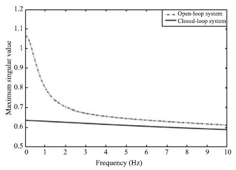
and using Algorithm 1,the desired static output feedback gain matrix is obtained as $K=0.1370$. We can easily compute and find that closed-loop system has the stable eigenvalues $\lambda_1$ $= -8.7288$,$\lambda_2=-34.4677$. In addition,with the designed controller,Fig. 1 shows the $H_\infty$ norm of the closed-loop system is smaller than thant of open-loop system.

Example 2. Consider the system (1) with the following parameters:

\begin{align*} &A=\left[\begin{array}{cc} -2.01 & 0\\0 & -5.3\end{array}\right],\ \ B_1=\left[ \begin{array}{c} -5\\ 0.5 \end{array} \right],\\[1mm] & B=\left[ \begin{array}{c} 0.2\\ 0.5 \end{array} \right],\ \ C=\left[ \begin{array}{cc} 0.99&1.01 \end{array} \right],\\[1mm] &C_y=\left[ \begin{array}{cc} 1.01&1.89 \end{array} \right],\ \ D=0.58,\ \ \alpha=1.2. \end{align*}

When $w(t)=0$,it is easy to see such system is asymptotically stable. Thus,in the following setting,we mainly make the comparison of $H_\infty$ norm of closed loop system over different frequency ranges. Firstly,for different frequency ranges,we adopt same initial matrix $U=[-0.2923\ 0.1175]$ which can be obtained by solving LMI (12). 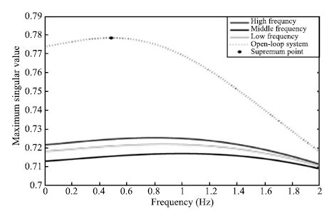Then we can design the different desired static output feedback controller using ILMI algorithm over three kinds of frequency ranges. After that,the norm values of the transfer function of the open-loop system and the closed-loop systems over three kinds of frequency ranges,are compared in Fig. 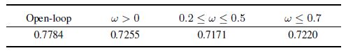2,and the $H_\infty$ norm comparison are presented in Table Ⅱ. From Fig. 2,we can see that controllers over three kinds of frequency ranges yield the smaller $H_\infty$ norm compared with the open loop system. From Table Ⅱ,we can see the least $H_\infty$ norm are generated by controller over the frequency range $[0.2 \ 0.5]$,which exactly is the range that the supremum point of maximum singular value of open loop system belongs to. Therefore,if the disturbance has a finite frequency,the minimization on the entire frequency range may not give the optimal solution. In order to achieve a better result in the optimization,it is meaningful to investigate the finite frequency $H_\infty$ control.

Ⅴ. Conclusions

In this paper,the $H_\infty$ output feedback control problem of fractional-order systems over finite frequency range has been investigated. Based on the GKYP Lemma and the Projection Lemma,we have established the existence conditions of the desired static output feedback controller. By matrix congruence transformation, the feedback gain matrix is decoupled with three matrix variables simultaneously,and further parameterized by a scalar matrix. Two iterative LMI algorithms have been presented to obtain the desired results. Furthermore,the existence conditions of desired controller have been extended to the high frequency and low frequency cases. Moreover,the design method is feasible for the fractional order $\alpha\in(1,2)$ case. Finally,numerical examples are given to show the effectiveness of our design method.