 2016, Vol.3


2. College of Automation, Chongqing University, Chongqing 400044, China
Complex networks widely exist in the world,from Internet to World Wide Web,from communication networks to social network,etc.. All the above networks can be represented in terms of nodes and edges,where edges indicate connections between nodes. Due to the tremendous potentials in real applications,the research of complex networks has become a hot topic in modern scientific research[1, 2, 3, 4]. In recent years,synchronization in complex network,as collective behavior,has received increasing attention and been extensively investigated due to its potential applications in many fields,including secure communization,image processing, neural networks,information science,etc.[5, 6, 7, 8, 9]. However,there exists much uncertain information in real-world complex networks[10, 11],such as the unknown or uncertain topological structure and node dynamics,as it is often difficult to exactly know all system parameters beforehand in many practical applications. Moreover,the uncertainty would greatly affect the modeling,understanding and controlling of the complex networks. Therefore,the issue of network structure and parameter identification is of theoretical and practical importance for uncertain complex dynamical networks. However,due to the nonlinear, complex,and high dimensional nature of the practical complex networks,it is very difficult to exactly identify its topological structure and system parameters by using the traditional approaches. Recently,some researchers have made great effort to address this problem and some valuable results have been obtained[12, 13, 14]. Wu[12] proposed an adaptive feedback control method to identify the exact topology of weighted general complex dynamical networks with time delay. Zhou et al.[13] investigated the topology identification of weighted complex dynamical networks. Liu et al.[14] proposed a novel adaptive feedback control approach to simultaneously identify the unknown or uncertain network topological structure and system parameters of uncertain delayed general complex dynamical networks. It is noted that the mentioned references [12, 13, 14] mainly contribute to the control or identification of networks with nodes of conventional integer-order dynamics.
On the other hand,the study of complex network with fractional-order dynamic nodes also begins to attract increasing interest among the researchers. It is well known that the fractional calculus is a classical mathematical notion,and is a generalization of ordinary differentiation and integration to arbitrary order[15]. However,the fractional calculus did not attract much attention for a long time due to lack of application background. Nowadays,many known systems can be described by fractional-order systems,such as viscoelastic system,dielectric polarization,electromagnetic waves[16, 17, 18]. Compared with the classical integer-order models,fractional-order derivatives provide an excellent instrument for the description of memory and hereditary properties of various materials and processes. Therefore,it may be more accurate to model by fractional-order derivatives than integer-order ones. It is demonstrated that many fractional-order differential systems behave chaotically or hyperchaotically,such as the fractional-order Chua circuit[19],the fractional-order Lorenz system[20],the fractional-order chaotic and hyperchaotic RÖssler system[21],etc.. Following these findings,synchronization of chaotic fractional-order differential systems becomes a challenging and interesting problem due to the potential applications in secure communication and control processing.
Not surprisingly, a complex network with nodes modeled by fractional-order differential systems has currently been one of the most promising research topics. However, due to the limited, theories, for, the , coupled, fractional-order, dynamical systems,the synchronization between fractional-order complex networks is still a challenging research topic. Compared with integer-order complex networks,the fractional-order complex networks related studies are still few[22, 23, 24, 25, 26, 27, 28, 29]. For example,Chai et al.[22] investigated synchronization of general fractional-order complex dynamical networks by adaptive pinning method. In [22, 23, 24, 25], the authors discussed the cluster synchronization in fractional-order complex networks. Wu and Lu[26] investigated outer synchronization between two different fractional-order general complex networks. The above mentioned literatures concentrated on the research of fractional-order network with known system parameters and network structures. So far,there are very few studies on the parameter estimation and topology identification of uncertain fractional-order complex networks.
Time delay is ubiquitous in many physical systems due to the finite switching speed of amplifiers,the finite signal propagation time in biological networks,traffic congestions and so forth. Time delay in the interaction may influence the dynamical behavior of the system. Si et al.[27] has investigated the identification of fractional-order complex network with unknown system parameters and network topologies. Yang and Jiang[28] has discussed the drive-response fractional-order complex dynamical network with uncertainty. Unfortunately,time delay is ignored. Although Ma et al.[29] discussed parameter identification and synchronization problem of fractional-order neural networks with time delays,but only the case of state variables $x \in {\bf R}$ is discussed,and the case for state vector $x$ $\in$ ${\bf R}^n$ has not been investigated.
Motivated by the above discussion,in this paper,we will study the identification of unknown system parameters and network topologies in uncertain fractional-order complex network with coupling delay and node delay. The paper is organized as follows. In Section Ⅱ, some fractional-order definitions and lemmas are given. Sections Ⅲ and Ⅵ study the parameter estimation and topology identification method for delayed fractional-order complex networks with different nodes. In Section V,two representative examples are given to demonstrate the effectiveness of the proposed method. Finally,some concluding remarks are given in Section Ⅵ.
Throughout this paper,the following notations are used. $\left\| \cdot \right\|$ is the Euclidean norm of a vector. $A^{\rm T}$ means the transpose of the matrix $A$. $I_n$ denotes the identity matrix with dimension $n$. $ \otimes $ represents the Kronecker product of two matrices.
Ⅱ. Preliminaries and notations A. The Definition of Fractional Calculus
The fractional-order integer-differential operator is the
generalized concept of an integer-order integer-differential
operator,which is denoted by a fundamental operator as follows:
\begin{align}
{ }_aD_t^q = \begin{cases}
\dfrac{{\rm d}^q}{{\rm d}t^q},& R\left( q \right) > 0,
\\[3mm]
1,& R\left( q \right) = 0,\\[1mm]
\int_a^t {\left( {{\rm d}\tau } \right)} ^{ - q},& R\left( q \right) < 0,
\end{cases}
\end{align}
(1)
Definition 1. The Caputo fractional derivative is defined
as follows
\begin{align}
D^q x(t) \buildrel\textstyle.\over= { }_a^c D_t^q x(t) =
\begin{cases}
\frac{1}{\Gamma (n - q)}\int_a^t (t - \tau )^{n - q - 1}x^{(n)}(\tau
){\rm d}\tau ,\\
\qquad\qquad\qquad\qquad\ \ \,n - 1 < q < n,\\[2mm]
\dfrac{{\rm d}^n}{{\rm d}t^n}x(t),\qquad\qquad\qquad\qquad\ \,q =
n,
\end{cases}
\end{align}
(2)
It should be noted that the advantage of the Caputo approach is that the initial conditions for fractional differential equations with Caputo derivatives take on the same form as those for integer-order ones,which have well understood physical meaning. Therefore,in the rest of this paper,the notation $\dfrac{{\rm d}^q}{{\rm d}t^q}$ is chosen as the Caputo fractional derivation operator.
B. Mathematical Preliminaries
Consider uncertain dynamical systems
\begin{align}
D^qx_i (t) = \bar f _i (t,x_i (t),\alpha _i ),
\end{align}
(3)
\begin{align}
D^qx_i (t) = f_i (t,x_i (t)) + F_i (t,x_i (t))\alpha _i,
\end{align}
(4)
Assumption 1. Suppose that there exist positive
constants $L_i$ such that
\begin{align}
\left\| {\bar f _i (t,x(t),\alpha _i ) - \bar f _i (t,y(t),\alpha
_i )} \right\| \le L_i \left\| {x(t) - y(t)} \right\|,
\end{align}
(5)
Assumption 2. Denote $F_i ( t,x_i ( t ) ) =( F_i ^{( 1 )}(t,x_i ( t ))$,$F_i ^{( 2 )}(t,x_i ( t )),\ldots ,F_i ^{( {m_i } )}(t,x_i ( t )) )$. Suppose that $F_i ^{( j )}( t$,$x_i ( t ) )$ $\in$ ${\bf R}^n$ for $j = 1,2,\ldots,m_i $,and $\{ \{ {F_i ^{( j )}( {t,x_i ( t )} )} \}_{j = 1}^{m_i } $,$\{ Ax_j ( t -\tau ) \}_{j = 1}^N \}$ are linearly independent on the orbit $\{ x_i ( t )$,$x_i ( {t - \tau } ) \}_{i = 1}^N $ of synchronization manifold.
If time delay $\tau $ is considered,similar to (3) and (4),we
can get the following delayed uncertain dynamical systems:
\begin{align}
D^qx_i (t) = \bar g _i (t,x_i (t),x_i \left( {t - \tau }
\right),\beta_i ),{\kern 1pt} {\kern 1pt} {\kern 1pt} {\kern 1pt}
\mbox{ }i = 1,2,\ldots.,N,
\end{align}
(6)
\begin{align}
D^qx_i (t)=&\ \bar {g}_i \left( {t,x_i (t),x_i \left( {t - \tau }\right),\beta _i } \right)
\notag\\[1mm]
=&\ g_i \left( {t,x_i \left( t \right),x_i \left(
{t - \tau } \right)} \right) \notag\\[1mm]
& + G_i \left( {t,x_i \left( t \right),x_i \left(
{t - \tau } \right)} \right)\beta _i ,
\end{align}
(7)
Assumption 3. Assume that there exists a
nonnegative constant $M$ satisfying
\begin{align}
&\left\| {\bar {g}_i \left( {t,x\left( t \right),x\left( {t - \tau
} \right),\beta _i } \right)} - {\bar {g}_i \left(
{t,y\left( t \right),y\left( {t - \tau } \right),\beta _i } \right)} \right\|\notag\\
&\qquad \le\sqrt M \left( {\left\| {x\left( t \right) - y\left( t
\right)}
\right\|^2 + \left\| {x\left( {t - \tau } \right) - y\left( {t - \tau }
\right)} \right\|^2} \right)^{\frac{1}{2}}. \end{align}
(8)
Lemma 1 [30] Consider a delayed fractional
order system:
\begin{align}
D^q x(t) = f\left( {x\left( t \right),x\left( {t - \tau }
\right)} \right),
\end{align}
(9)
\begin{align}
x^{\rm T}(t)P D^q x(t) + x^{\rm T}\left( t \right)Qx\left( t \right) - x^{\rm T}\left(
{t - \tau } \right)Qx\left( {t - \tau } \right) \le 0,
\end{align}
(10)
Lemma 2. [26] For any vector $x$,$y \in {\bf R}^n$,the inequality $2x^{\rm T}y$ $\le$ $x^{\rm T}x + y^{\rm T}y$ holds.
Ⅲ. Structure identification of uncertain general fractional-order complex dynamical networks with coupling delay
Consider a complex dynamical network with time-varying coupling
delay and $N$ different nodes,which is described by
\begin{align}
D^qx_i \left( t \right) = \bar f _i (t,x_i (t),\alpha _i ) +
\sum\limits_{j = 1}^N {c_{ij} Ax_j \left( {t - \tau } \right)} ,
\end{align}
(11)
\begin{align}
& D^qx_i \left( t \right) =\notag\\[1mm]
&\qquad f_i \left( {t,x_i \left( t \right)} \right) + F_i \left(
{t,x_i \left( t \right)} \right)\alpha _i + \sum\limits_{j = 1}^N
{c_{ij} Ax_j \left( {t - \tau } \right)} ,
\end{align}
(12)
Hereafter,the coupling configuration matrix $C$ need not be symmetric,irreducible,or diffusive. Of course,it is necessary to ensure the boundedness of complex dynamical networks in this paper. The main goal is to identify these unknown or uncertain coupling strengths,namely the network topological structure,and all unknown system parameter vectors $\alpha _i $ of the complex dynamical networks.
Consider another complex dynamical network which will be referred
to as the response network with coupling delay as follows:
\begin{align}
D^q\hat {x}_i \left( t \right) =&\ f_i \left( {t,\hat {x}_i \left( t
\right)}
\right) + F_i \left( {t,\hat {x}_i \left( t \right)} \right)\hat {\alpha }_i\notag\\
&\,+\sum\limits_{j = 1}^N {\hat {c}_{ij} A\hat {x}_j \left( {t -
\tau }
\right) + u_i } ,
\end{align}
(13)
Denote $\tilde {x}_i = \hat {x}_i - x_i $,$\tilde {c}_{ij} = \hat
{c}_{ij} - c_{ij} $,$\tilde {\alpha }_i = \hat {\alpha }_i - \alpha
_i $. The systems (12) and (13) achieve synchronization if $\tilde
{x}_i \to 0$ as $t$ $\to$ $\infty $. Then the error system is given
by
\begin{align}
\tilde {x}_i (t) = &\ f_i ( {t,\hat {x}_i (t)} ) + F_i ( {t,\hat
{x}_i (t)} )\hat {\alpha }_i - f_i (t,x_i ( t
) )\notag\\
&\,-F_i ( t,x_i (t) )\alpha _i
+ \sum\limits_{j = 1}^N \hat{c}_{ij} A\hat {x}_j ( t -
\tau )\notag\\
&\,- \sum\limits_{j = 1}^N c_{ij} Ax_j ( t - \tau
) + u_i.
\end{align}
(14)
| \begin{align} D^q\tilde {x}_i (t) =&\ \bar {f}_i\left( {t,\hat {x}_i \left( t \right),\alpha _i } \right) - \bar {f}_i \left( {t,x_i (t),\alpha _i } \right)\notag\\ &\,+ F_i \left( {t,\hat {x}_i (t)} \right)\tilde {\alpha }_i + \sum\limits_{j = 1}^N \tilde {c}_{ij} A\hat {x}_j \left( {t - \tau } \right)\notag\\ &\,-\sum\limits_{j = 1}^N {c_{ij} A\tilde {x}_j \left( {t - \tau } \right) + u_i } . \end{align} | (15) |
Theorem 1. Suppose that Assumptions A1 and A2 hold. Then
the uncertain coupling configuration matrix $C$ and parameter
vectors $ \alpha _i$ of uncertain general delayed complex dynamical
network (12) can be identified by the estimated values $\hat {C}$
and $\hat {\alpha }_i$ via the response network
\begin{align}
\begin{cases}
D^q\hat {x}_i = f_i \left( {t,\hat {x}_i (t)} \right) + F_i \left( {t,\hat
{x}_i \left( t \right)} \right)\hat {\alpha }_i \\
\qquad \quad \ +\sum\limits_{j = 1}^N
{\hat {c}_{ij} A\hat {x}_j \left( {t - \tau } \right) + u_i ,}
\\[1mm]
u_i = - k_i \tilde {x}_i \left( t \right),{\kern 1pt} {\kern 1pt} {\kern
1pt} {\kern 1pt} {\kern 1pt} {\kern 1pt} \\[1mm]
D^qk_i = d_i \left\| {\tilde {x}_i } \right\|^2,\\[1mm]
D^q\hat {\alpha }_i = - F_i ^{\rm T}\left( {t,\hat {x}_i \left( t \right)}
\right)\tilde {x}_i \left( t \right),\\[1mm]
D^q\hat {c}_{ij} = - \delta _{ij} \tilde {x}_i \left( t \right)^{\rm T}A\hat
{x}_j \left( {t - \tau } \right),
\end{cases}
\end{align}
(16)
Proof. Denote $\tilde {k}_i = k_i - k_i^* $,and $k_i^*$
is a positive constant. Further denote $X = ( {\tilde {X}^{\rm
T},\tilde {\alpha }^{\rm T},\tilde {c}^{\rm T},\tilde
{k}^{\rm T}} )^{\rm T}$,where
\begin{align}
\begin{cases}
\tilde {X} = \left( {\tilde {x}^{\rm T}_1 ,\tilde {x}^{\rm T}_2 ,\ldots,\tilde {x}^{\rm T}_N }
\right)^{\rm T},~~\tilde {x}_i = \left( {\tilde {x}_{i1} ,\tilde {x}_{i2}
,\ldots,\tilde {x}_{in} } \right)^{\rm T},\\[1mm]
\tilde {\alpha } = \left( {\tilde {\alpha }^{\rm T}_1 ,\tilde {\alpha }^{\rm T}_2
,\ldots,\tilde {\alpha }^{\rm T}_N } \right)^{\rm T},~~\tilde {\alpha }_i = \left( {\tilde
{\alpha }_{i1} ,\tilde {\alpha }_{i2} ,\ldots,\tilde {\alpha }_{im_i } }
\right)^{\rm T},\\[1mm]
\tilde {c} = \left( {\tilde {c}_1 ^{\rm T},\tilde {c}_2 ^{\rm T},\ldots,\tilde {c}_N ^{\rm T}}
\right)^{\rm T},~~~~\,\tilde {c}_i = \left( {\tilde {c}_{i1} ,\tilde {c}_{i2} ,\ldots,\tilde
{c}_{iN} } \right)^{\rm T},\\[1mm]
\tilde {k} = \left( {\tilde {k}_1 ,\tilde {k}_2 ,\ldots,\tilde {k}_N }
\right)^{\rm T}.
\end{cases}
\end{align}
(17)
\begin{align}
&P = {\rm{diag}} \left\{{\underbrace
{1,\ldots,1}_{nN+\sum\limits_{i = 1}^N {{m_i}} },\frac{1}{\delta
_{11}
},\ldots,\frac{1}{\delta _{NN} },\frac{1}{d_1
},\ldots,\frac{1}{d_N }} \right\},\\
&Q = {\rm{diag}} \left\{ {\underbrace
{1,\ldots,1}_{nN},\underbrace {0,\ldots,0}_{\sum\limits_{i = 1}^N
{{m_i}} +N^2+N}} \right\}.
\end{align}
(18)
\begin{align*}
J=&\ X^{\rm T}(t)PD^qX(t) + X^{\rm T}\left( t \right)QX\left( t \right)\\
&\,-X^{\rm T}\left( {t - \tau } \right)QX\left( {t - \tau } \right)\\
=&\ \sum\limits_{i = 1}^N \tilde {x}^{\rm T}_i \left( t
\right)D^q\tilde {x}_i\left( t \right) + \sum\limits_{i
= 1}^N \tilde {\alpha }_i ^{\rm T}D^q\tilde {\alpha }_i
\\& \,+ \sum\limits_{i = 1}^N \sum\limits_{j = 1}^N
\frac{1}{\delta _{ij} }\tilde {c}_{ij} D^q\tilde {c}_{ij}
+ \sum\limits_{i = 1}^N
{\frac{1}{d_i }\tilde {k}_i D^q\tilde {k}_i } \\
&\,+\sum\limits_{i = 1}^N {\tilde {x}_i
^{\rm T}(t)\tilde {x}_i \left( t \right) - \sum\limits_{i = 1}^N {\tilde {x}_i
^{\rm T}(t - \tau )\tilde {x}_i \left( {t - \tau } \right)} } \\
=&\ \sum\limits_{i = 1}^N \tilde {x}_i ^{\rm T}(t)\left\{ {\bar
{f}_i \left(
{t,\hat {x}_i \left( t \right),\alpha _i } \right) - \bar {f}_i \left(
{t,x_i (t),\alpha _i } \right)} \right\}\\
&\,+\sum\limits_{i = 1}^N {\tilde
{x}_i ^{\rm T}\left( t \right)F_i \left( {t,\hat {x}_i \left( t \right)}
\right)\tilde {\alpha }_i } \\
&\,+\sum\limits_{i = 1}^N \sum\limits_{j = 1}^N
c_{ij} \tilde {x}_i ^{\rm T}\left( t \right)A\tilde {x}_j \left( {t - \tau }
\right) - \sum\limits_{i = 1}^N k_i \left\| {\tilde {x}_i \left( t \right)}
\right\|^2 \\
&\,+\sum\limits_{i = 1}^N {\sum\limits_{j = 1}^N {\tilde {c}_{ij}
\tilde {x}_i ^{\rm T}\left( t \right)A\hat {x}_j \left( {t - \tau } \right)} } \\
&\,+\sum\limits_{i
= 1}^N \tilde {\alpha }_i ^{\rm T}D^q\tilde {\alpha }_i
+ \sum\limits_{i = 1}^N \sum\limits_{j = 1}^N
\frac{1}{\delta _{ij} }\tilde {c}_{ij} D^q\tilde {c}_{ij}\\
&\,+\sum\limits_{i = 1}^N
{\left( {k_i - k^ * } \right)\left\| {\tilde {x}_i \left( t \right)}
\right\|^2} \\
&\,+\sum\limits_{i = 1}^N {\tilde {x}_i ^{\rm T}(t)\tilde {x}_i
\left( t
\right) - \sum\limits_{i = 1}^N {\tilde {x}_i ^{\rm T}(t - \tau )\tilde {x}_i
\left( {t - \tau } \right)} } \\
\le&\ \sum\limits_{i = 1}^N L_i \tilde {x}_i ^{\rm T}\left( t
\right)\tilde
{x}_i (t)\\
&\,+ {\sum\limits_{i = 1}^N {\tilde {x}_i \left( t \right)F_i
\left( {t,\hat {x}_i \left( t \right)} \right)\tilde {\alpha }_i +
\sum\limits_{i = 1}^N {\tilde {\alpha }_i ^{\rm T}D^q\tilde {\alpha }_i } } } \\
&\,+\sum\limits_{i = 1}^N {\sum\limits_{j = 1}^N {{{\tilde c}_{ij}}\tilde x_i^{\rm T}\left( t \right)A{{\hat x}_j}\left( {t - \tau } \right)} } \\
&\,+\sum\limits_{i = 1}^N {\sum\limits_{j = 1}^N {\frac{1}{{{\delta
_{ij}}}}{{\tilde c}_{ij}}{D^q}{{\tilde c}_{ij}}} }
\end{align*}
\begin{align}
&\,+\sum\limits_{i= 1}^N \sum\limits_{j = 1}^N c_{ij} \tilde {x}_i
^{\rm T}\left( t \right)A\tilde
{x}_j ( t - \tau ) - \sum\limits_{i = 1}^N k^ * \left\| \tilde {x}_i (t) \right\|^2\notag\\
&\,+\sum\limits_{i = 1}^N {\tilde
{x}_i ^{\rm T}(t)\tilde {x}_i \left( t \right) - \sum\limits_{i = 1}^N {\tilde
{x}_i ^{\rm T}(t - \tau )\tilde {x}_i \left( {t - \tau } \right)} } \notag\\
\le &\ \sum\limits_{i = 1}^N \tilde {x}_i ^{\rm T}( t )\tilde {x}_i
( t ) + \sum\limits_{i = 1}^N \sum\limits_{j = 1}^N c_{ij}
\tilde {x}_i ( t )A\tilde {x}_j ( {t - \tau} ) \notag\\
& \,-\sum\limits_{i = 1}^N {k^ * \left\| {\tilde {x}_i \left(
t \right)} \right\|^2} + \sum\limits_{i = 1}^N \tilde {x}_i ^{\rm T}(t)\tilde {x}_i \left( t
\right) \notag\\
&\,- \sum\limits_{i = 1}^N {\tilde {x}_i ^{\rm T}(t - \tau )\tilde
{x}_i
\left( {t - \tau } \right),} \notag\\
\le &\ L\tilde {X}^{\rm T}(t)\tilde {X}(t) + \tilde {X}^{\rm T}(t)(C
\otimes A)\tilde {X}(
{t - \tau } )\notag\\
&\,- k^ * \tilde {X}^{\rm T}( t)\tilde {X}( t )+ \tilde {X}^{\rm T}(t )\tilde {X}( t) \notag\\
&\,-\tilde {X}^{\rm T}( t - \tau )\tilde {X}( t - \tau) \notag\\
\le&\ L\tilde {X}^{\rm T}( t )\tilde {X}( t ) +
\frac{1}{2}\tilde {X}^{\rm T}( t )(CC^{\rm T} \otimes AA^{\rm T})\tilde {X}( t ) \notag\\
&\,+ \frac{1}{2}\tilde {X}^{\rm T}( t - \tau)\tilde {X}( t - \tau )
- k^ * \tilde {X}^{\rm T}( t
)\tilde {X}( t )\notag\\
&\,+\tilde {X}^{\rm T}( t )\tilde {X}( t) - \tilde {X}^{\rm T}( t -
\tau )\tilde {X}(
t - \tau ) \notag\\
=&\ \left( {L - k^ * + 1 + \frac{1}{2}\lambda _{\max }
{(CC^{\rm T} \otimes AA^{\rm T})} } \right)\tilde {X}^{\rm T}(t)\tilde {X}(t) \notag\\&\,- \frac{1}{2}\tilde {X}^{\rm T}\left( {t - \tau }
\right)\tilde {X}\left( {t - \tau } \right),
\end{align}
(20)
Remark 1. It should be especially pointed out that the coupling configuration matrix $C$ need not be symmetric, irreducible, even diffusive.
Remark 2. The positive constants $\delta _{ij} $,$d_i $ in the updating laws $D^qk_i $ and $D^q\hat {c}_{ij} $ can control the convergence speed of the synchronization and identification.
Remark 3. Assumption A2 is a very essential condition for guaranteeing the success of identification. Without this condition, it may cause false identification result. Similarly,Assumption A4 guarantees the identification of the next section.
Ⅳ. Structure identification of an uncertain general complex dynamical network with node delay
Consider an uncertain general complex dynamical network consisting
of $ N $ different nodes with time delay $\tau $,called the drive
network,which is described by
\begin{align}
D^qx_i (t) = \bar {g}_i \left( {t,x_i (t),x_i \left( {t - \tau
}\right),\beta _i } \right) + \sum\limits_{j = 1}^N c_{ij} Ax_j
(t),
\end{align}
(21)
\begin{align}
&\bar {g}_i \left( {t,x_i (t),x_i \left( {t - \tau } \right),\beta
_i } \right)\notag\\ &\qquad =g_i \left( {t,x_i \left( t
\right),x_i \left( {t - \tau } \right)} \right) + G_i \left( {t,x_i
\left( t \right),x_i \left( {t - \tau } \right)} \right)\beta _i,
\end{align}
(22)
Construct another controlled general fractional-order complex
network,called response network,which is given by
\begin{align}
D^q\hat {x}_i = \bar {g}_i \left( {t,\hat {x}_i (t),\hat {x}_i
\left( {t - \tau } \right),\hat {\beta }_i } \right) +
\sum\limits_{j = 1}^N {\hat
{c}_{ij} A\hat {x}_j (t)} + u_i ,%\\ i = 1,\ldots,N,
\end{align}
(23)
| \begin{align} D^q\tilde {x}_i \left( t \right) =&\ \bar {g}_i \left( {t,\hat {x}_i \left( t \right),\hat {x}_i \left( {t - \tau } \right),\beta _i } \right)\notag\\ &\,-\bar {g}_i \left( {t,x_i \left( t \right),x_i \left( {t - \tau } \right),\beta _i } \right) \notag\\ &\,+ G_i \left( {t,\hat {x}_i \left( t \right),\hat {x}_i \left( {t - \tau } \right)} \right)\tilde {\beta }_i \notag\\ &\,+ \sum\limits_{j = 1}^N {\tilde {c}_{ij} A\hat {x}_j \left( t \right)} + \sum\limits_{j = 1}^N {c_{ij} A\tilde {x}_j \left( t \right) + u_i.} \end{align} | (24) |
Theorem 2. Suppose that Assumptions A3 and A4 hold. Then
uncertain coupling configuration matrix $C$ and system parameter
vectors $\beta _i$ can be identified by using the estimated values
$\hat {C}$ and $\hat {\beta}_i$ via the response network
\begin{align}
\begin{cases}
D^q\hat {x}_i \left( t \right) = g_i \left( {t,\hat {x}_i \left( t
\right),\hat {x}_i \left( {t - \tau } \right)} \right)\\
\qquad +~ G_i \left( {t,\hat
{x}_i \left( t \right),\hat {x}_i \left( {t - \tau } \right)} \right)\hat
{\beta }_i+
\sum\limits_{j = 1}^N \hat {c}_{ij} A\hat {x}_j \left( t \right) + u_i ,\\
u_i = - k_i \tilde {x}_i \left( t \right),\\
D^qk_i = d_i \left\| {\tilde {x}_i \left( t \right)} \right\|^2,\\
D^q\hat {\beta }_i = - G_i ^{\rm T}\left( {t,\hat {x}_i \left( t \right),\hat
{x}_i \left( {t - \tau } \right)} \right)\tilde {x}_i \left( t \right),\\
D^q\hat {c}_{ij} = - \delta _{ij} \tilde {x}_i ^{\rm T}\left( t \right)A\hat
{x}_j \left( t \right),
\end{cases}
\end{align}
(2)
Proof. Denote $\tilde {k}_i = k_i - k_i ^ * $,$k_i ^ * $
is a positive constant. Further denote $X = ( {\tilde {X}^{\rm
T},\tilde {\beta }^{\rm T},\tilde {c}^{\rm T},\tilde
{k}^{\rm T}})^{\rm T}$,where
\begin{align}
\begin{cases}
\tilde {X} = \left( {\tilde {x}^{\rm T}_1 ,\tilde {x}^{\rm T}_2 ,\ldots,\tilde {x}^{\rm T}_N }
\right)^{\rm T},~~\tilde {x}_i = \left( {\tilde {x}_{i1} ,\tilde {x}_{i2}
,\ldots,\tilde {x}_{in} } \right)^{\rm T},\\
\tilde {\beta } = \left( {\tilde {\beta }^{\rm T}_1 ,\tilde {\beta }^{\rm T}_2
,\ldots,\tilde {\beta }^{\rm T}_N } \right)^{\rm T},~~\tilde {\beta }_i = \left( {\tilde
{\beta }_{i1} ,\tilde {\beta }_{i2} ,\ldots,\tilde {\beta }_{im_i } }
\right)^{\rm T},\\
\tilde {c} = \left( {\tilde {c}_1 ^{\rm T},\tilde {c}_2 ^{\rm T},\ldots,\tilde {c}_N ^{\rm T}}
\right)^{\rm T},~~~~\,\tilde {c}_i = \left( {\tilde {c}_{i1} ,\tilde {c}_{i2} ,\ldots,\tilde
{c}_{iN} } \right)^{\rm T},\\
\tilde {k} = \left( {\tilde {k}_1 ,\tilde {k}_2 ,\ldots,\tilde {k}_N }
\right)^{\rm T}.
\end{cases}
\end{align}
(26)
\begin{align}
&P = {\rm{diag}}\left( {\underbrace {1,\ldots,1}_{nN+\sum\limits_{i
= 1}^N {{m_i}} },\frac{1}{\delta _{11}
},\ldots,\frac{1}{\delta _{NN} },\frac{1}{d_1
},\ldots,\frac{1}{d_N }} \right),
\end{align}
(27)
\begin{align}
&Q = {\rm{diag}} \left( {\underbrace
{\frac{M}{2},\ldots,\frac{M}{2}}_{nN},\underbrace
{0,\ldots,0}_{\sum\limits_{i = 1}^N {{m_i}} +N^2+N}} \right).
\end{align}
(28)
| \begin{align*} J=&\ X^{\rm T}(t)P D^q X(t) + X^{\rm T}\left( t \right)QX\left( t \right)\\ &\,-X^{\rm T}\left( {t - \tau } \right)QX\left( {t - \tau } \right)\\ =&\ \sum\limits_{i = 1}^N \tilde {x}_i ^{\rm T}\left( t \right)D^q\tilde {x}_i \left( t \right) + \sum\limits_{i = 1}^N \tilde {\beta }_i ^{\rm T}D^q\tilde {\beta }_i\\ &\,+ \sum\limits_{i = 1}^N {\sum\limits_{j = 1}^N {\frac{1}{\delta _{ij} }\tilde {c}_{ij} D^q\tilde {c}_{ij} } } + \sum\limits_{i = 1}^N \frac{1}{d_i }\tilde {k}_i D^qk_i \\ &\,+\sum\limits_{i = 1}^N {\frac{M}{2}\tilde {x}_i ^{\rm T}\left( t \right)\tilde {x}_i \left( t \right) - \sum\limits_{i = 1}^N {\frac{M}{2}\tilde {x}_i ^{\rm T}\left( {t - \tau } \right)\tilde {x}_i \left( {t - \tau } \right)} }\\ =&\ \sum\limits_{i = 1}^N {\tilde {x}_i ^{\rm T}\left( t \right)(} \bar {g}_i \left( {t,\hat {x}_i \left( t \right),\hat {x}_i \left( {t - \tau } \right),\beta _i } \right)\\ &\,-\bar {g}_i \left( {t,x_i \left( t \right),x_i \left( {t - \tau } \right),\beta _i } \right) \\ &\,+G_i \left( {t,\hat {x}_i \left( t \right),\hat {x}_i \left( {t - \tau } \right)} \right)\tilde {\beta }_i\\ &\,+ \sum\limits_{j = 1}^N {\tilde {c}_{ij} A\hat {x}_j \left( t \right)} + \sum\limits_{j = 1}^N {c_{ij} A\tilde {x}_j \left( t \right) - k_i \tilde {x}_i \left( t \right)} ) \\ &\,- \sum\limits_{i = 1}^N {\tilde {\beta }_i ^{\rm T}G_i ^{\rm T}\left( {t,\hat {x}_i \left( t \right),\hat {x}_i \left( {t - \tau } \right)} \right)\tilde {x}_i \left( t \right)}\\ &\,- \sum\limits_{i = 1}^N {\sum\limits_{j = 1}^N {\tilde {c}_{ij} \tilde {x}_i ^{\rm T}\left( t \right)A\hat {x}_j \left( t \right)} } + \sum\limits_{i = 1}^N {\left( {k_i - k^\ast } \right)\left\| {\tilde {x}_i ^{\rm T}\left( t \right)} \right\|^2} \\ &\,+ \sum\limits_{i = 1}^N {\frac{M}{2}\tilde {x}_i ^{\rm T}\left( t \right)\tilde {x}_i \left( t \right) - \sum\limits_{i = 1}^N {\frac{M}{2}\tilde {x}_i ^{\rm T}\left( {t - \tau } \right)\tilde {x}_i \left( {t - \tau } \right)} }\\ =& \ \sum\limits_{i = 1}^N \tilde {x}_i ^{\rm T}( t )( \bar {g}_i ( {t,\hat {x}_i ( t ),\hat {x}_i ( {t - \tau } ),\beta _i } )\\ &\,- \bar {g}_i ( {t,x_i ( t ),x_i ( {t - \tau } ),\beta _i } ) )\\ &\,+\sum\limits_{i = 1}^N \sum\limits_{j = 1}^N \tilde {x}_i ^{\rm T}\left( t \right)c_{ij} A\tilde {x}_j \left( t \right) - k^\ast \sum\limits_{j = 1}^N \left\| {\tilde {x}_i \left( t \right)} \right\|^2 \\ &\,+\sum\limits_{i = 1}^N \frac{M}{2}\tilde {x}_i ^{\rm T}\left( t \right)\tilde {x}_i \left( t \right) - \sum\limits_{i = 1}^N {\frac{M}{2}\tilde {x}_i ^{\rm T}\left( {t - \tau } \right)\tilde {x}_i \left( {t - \tau } \right)} \\ \le &\ \frac{\mbox{1}}{\mbox{2}}\sum\limits_{i = 1}^N \tilde {x}_i ^{\rm T}( t )\tilde {x}_i ( t ) + \frac{1}{2}\| \bar {g}_i ( {t,\hat {x}_i ( t ),\hat {x}_i ( {t - \tau } ),\beta _i } )\\ &\,-\bar {g}_i ( {t,x_i ( t ),x_i ( {t - \tau } ),\beta _i } ) \|^2 \\ &\,+\sum\limits_{i = 1}^N \sum\limits_{j = 1}^N \tilde {x}_i ^{\rm T}\left( t \right)c_{ij} A\tilde {x}_j \left( t \right) - k^\ast \sum\limits_{j = 1}^N \left\| {\tilde {x}_i \left( t \right)} \right\|^2 \\ &\,+\sum\limits_{i = 1}^N {\frac{M}{2}\tilde {x}_i ^{\rm T}\left( t \right)\tilde {x}_i \left( t \right) - \sum\limits_{i = 1}^N {\frac{M}{2}\tilde {x}_i ^{\rm T}\left( {t - \tau } \right)\tilde {x}_i \left( {t - \tau } \right)} } \\ \le &\ \frac{\mbox{1}}{\mbox{2}}\sum\limits_{i = 1}^N {\tilde {x}_i^{\rm T}\left( t \right)\tilde {x}_i \left( t \right) + \frac{M}{2}\left( {\left\| {\tilde {x}_i \left( t \right)} \right\|^2 + \left\| {\tilde {x}_i \left( {t - \tau } \right)} \right\|^2} \right)} \notag \end{align*} \begin{align} &\,+\sum\limits_{i = 1}^N {\sum\limits_{j = 1}^N {\tilde {x}_i ^{\rm T}\left( t \right)c_{ij} A\tilde {x}_j \left( t \right) - k^\ast \sum\limits_{j = 1}^N {\left\| {\tilde {x}_i \left( t \right)} \right\|^2 } } } \notag\\ &\,+ \sum\limits_{i = 1}^N \frac{M}{2}\tilde {x}_i ^{\rm T}\left( t \right)\tilde {x}_i \left( t \right) - \sum\limits_{i = 1}^N {\frac{M}{2}\tilde {x}_i ^{\rm T}\left( {t - \tau } \right)\tilde {x}_i \left( {t - \tau } \right)}\notag\\ =&\ \left( {\frac{1}{2} + M - k^\ast } \right)\tilde {X}^{\rm T}\left( t \right)\tilde {X}\left( t \right) + \tilde {X}^{\rm T}\left( t \right)\left( {C \otimes A} \right)\tilde {X}\left( t \right)\notag\\ \le&\ \left(\frac{1}{2} + M - k^\ast + \lambda_{\rm max} (C \otimes A) \right) \tilde {X}^{\rm T}(t)\tilde {X}( t ). \end{align} | (29) |
It is obvious that there exists sufficiently large positive constant $k^ * $ such that $J $ is negative definite. Namely,$X^{\rm T}(t)P$ $\times$ $D^qX(t)+X^{\rm T}(t)QX(t) - X^{\rm T}(t - \tau )QX(t - \tau ) \le 0$ holds,which implies the Lyapunov stability of error system (24) by Lemma 1.
Ⅴ. Numerical simulationsIn this section,two representative examples are given to verify the effectiveness of the proposed parameters estimation and structure identification approaches.
A. Identification with Coupling Time Delay
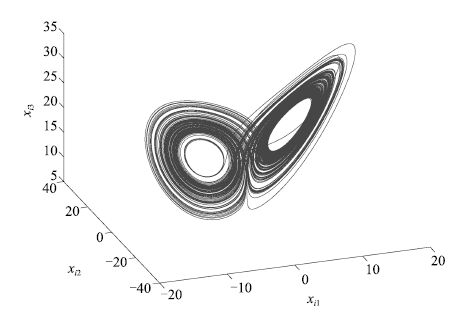
The well-known Lü system with fractional order derivative is
used as the node dynamics in the uncertain network,which is
described as
\begin{align}
D^qx_i (t) = f_i \left( {t,x_i \left( t \right)} \right) + F_i
\left( {t,x_i (t)} \right)\alpha _i ,
\end{align}
(30)

|
Download:
|
| Fig. 1 Chaotic attractor of fractional-order Lü system. | |
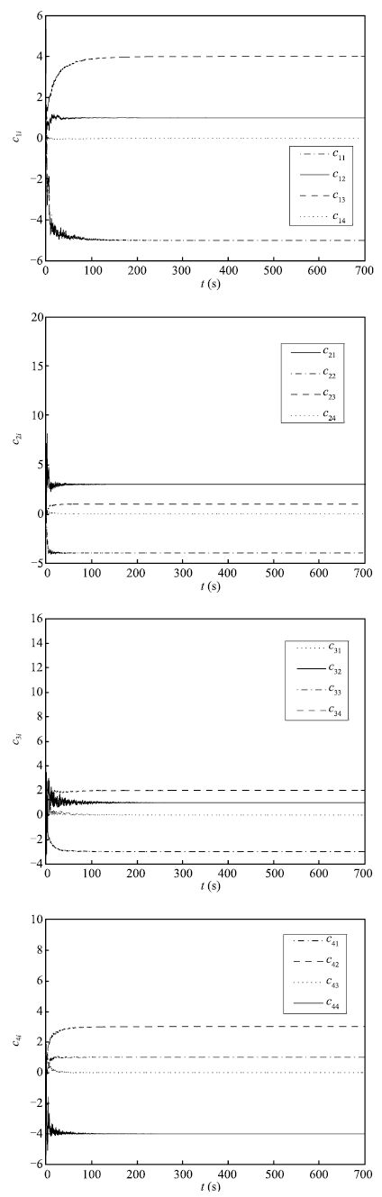
The weight configuration matrix is set as
\begin{align}
C=\left( {{\begin{array}{*{20}c}
{ - 5} \hfill & ~~1 \hfill & ~~4 \hfill & ~~0 \hfill \\
~~3 \hfill & { - 4} \hfill & ~~1 \hfill & ~~0 \hfill \\
~~0 \hfill & ~~1 \hfill & { - 3} \hfill & ~~2 \hfill \\
~~1 \hfill & ~~3 \hfill & ~~0 \hfill & { - 4} \hfill \\
\end{array} }} \right).
\end{align}
(31)
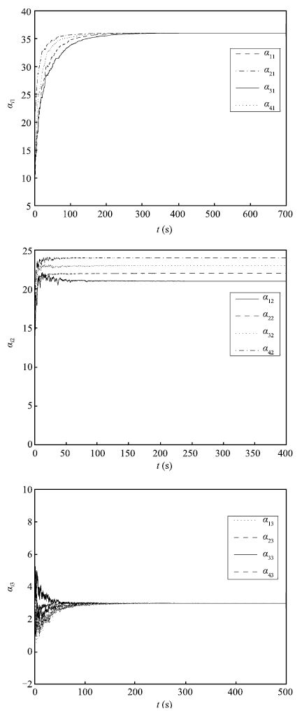
Let $\alpha _i = ( {\alpha _{i1} ,\alpha _{i2} ,\alpha _{i3} } )^{\rm T} = ( {36,{\kern 1pt} {\kern 1pt} {\kern 1pt} {\kern 1pt} 20 + i,{\kern 1pt} {\kern 1pt} {\kern 1pt} {\kern 1pt} 3} )^{\rm T}$ for $i =1,$ $\ldots,$ $4$. $\tau = 0.2$,and networks inner-coupling matrix $A=$ ${\rm{diag}}\{1,$ $1,$ $1\}$.
According to Theorem 1,the coupling configuration matrix $C$ and system parameter vectors $\alpha _i $ of complex networks (12) can be identified by using adaptive control laws (16). Fig. 2 shows the identification of the uncertain system parameters,while Fig. 3 illustrates the identification of the unknown network topology.

|
Download:
|
| Fig. 2 Identification of uncertain parameters. | |

|
Download:
|
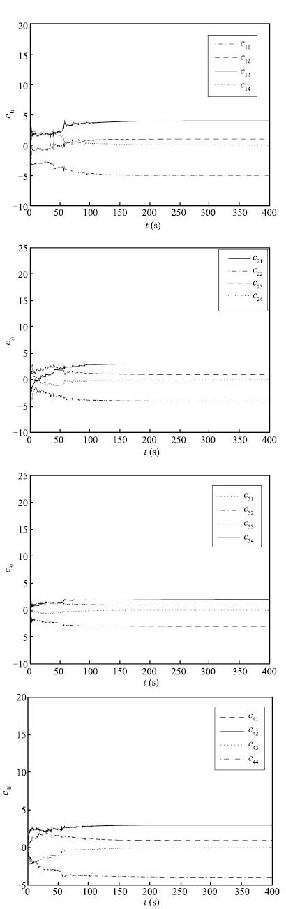
| Fig. 3 Identification of network structure. | |
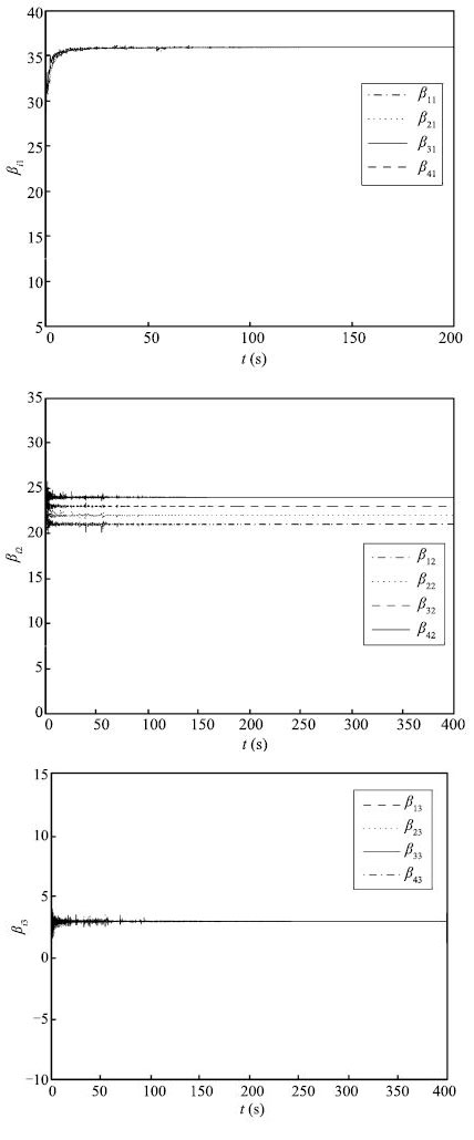
In this subsection,we consider the uncertain network (21) with four
nonidentical delayed Lü systems, and the single delayed Lü
system is described as
\begin{align}
\begin{cases}
D^qx_{i1} \left( t \right) = \beta _{i1} \left( {x_{i2} \left( {t - \tau }
\right) - x_{i1} \left( {t - \tau } \right)} \right),
\\[1.5mm]
D^qx_{i2} \left( t \right) = - x_{i1} \left( {t - \tau } \right)x_{i3}
\left( {t - \tau } \right) + \beta _{i2} x_{i2} \left( {t - \tau } \right),
\\[1.5mm]
D^qx_{i3} \left( t \right) = x_{i1} \left( {t - \tau } \right)x_{i2} \left(
{t - \tau } \right) - \beta _{i3} x_{i3} \left( {t - \tau } \right),
\end{cases}
\end{align}
(32)

|
Download:
|
| Fig. 5 Identification of uncertain parameters. | |

|
Download:
|
| Fig. 6 Identification of network structure. | |
In this paper,a novel and feasible approach to identify the parameters and network topology of fractional-order complex network with time delay is proposed. Based on the stability theorem of fractional-order differential system and the adaptive control technique,two useful identification criteria are derived. Illustrative simulations are provided to verify the correctness and effectiveness of the proposed methods.
| [1] | Strogatz S H. Exploring complex networks. Nature, 2001, 410(6825): 268-276 |
| [2] | Wang X F, Chen G R. Complex networks: small-world, scale-free and beyond. IEEE Circuits and Systems Magazine, 2003, 3(1): 6-20 |
| [3] | Boccaletti S, Latora V, Moreno Y, Chavez M, Hwang D U. Complex networks: structure and dynamics. Physics Reports, 2006, 424(4-5): 175-308 |
| [4] | Albert R, Barabási A L. Statistical mechanics of complex networks. Reviews of Modern Physics, 2002, 74(1): 47-97 |
| [5] | Chen G R, Dong X N. From Chaos to Order: Methodologies, Perspectives and Applications. Singapore: World Scientific, 1998. |
| [6] | Xie Q X, Chen G R, Bollt E M. Hybrid chaos synchronization and its application in information processing. Mathematical and Computer Modelling, 2002, 35(1-2): 145-163 |
| [7] | Li X, Wang X F, Chen G R. Pinning a complex dynamical network to its equilibrium. IEEE Transactions on Circuits and Systems I: Regular Papers, 2004, 51(10): 2074-2087 |
| [8] | Arenas A, Díaz-Guilera A, Kurths J, Moreno Y, Zhou C S. Synchronization in complex networks. Physics Reports, 2008, 469(3): 93-153 |
| [9] | Wu X J, Lu H T. Hybrid synchronization of the general delayed and non-delayed complex dynamical networks via pinning control. Neurocomputing, 2012, 89: 168-177 |
| [10] | Lu J Q, Cao J D. adaptive complete synchronization of two identical or different chaotic (hyperchaotic) systems with fully unknown parameters. Chaos, 2005, 15(4): 043901 |
| [11] | Yu D C, Righero M, Kocarev L. Estimating topology of networks. Physical Review Letters, 2006, 97(18): 188701 |
| [12] | Wu X Q. Synchronization-based topology identification of weighted general complex dynamical networks with time-varying coupling delay. Physica A: Statistical Mechanics and Its Applications, 2008, 387(4): 997-1008 |
| [13] | Zhou J, Lu J A. Topology identification of weighted complex dynamical networks. Physica A: Statistical Mechanics and Its Applications, 2007, 386(1): 481-491 |
| [14] | Liu H, Lu J A, Lü J H, Hill D J. Structure identification of uncertain general complex dynamical networks with time delay. Automatica, 2009, 45(8): 1799-1807 |
| [15] | Nagih A, Plateau G. Problémes fractionnaires: tour d'horizon sur les applications et méthodes de résolution. RAIRO-Operations Research, 1999, 33(4): 383-419 |
| [16] | Koeller R C. Applications of fractional calculus to the theory of viscoelasticity. Journal of Applied Mechanics, 1984, 51(2): 299-307 |
| [17] | Heaviside O. Electromagnetic Theory. New York: Chelsea, 1971. |
| [18] | Podlubny I. Fractional Differential Equations. San Diego: Academic Press, 1999. |
| [19] | Hartley T T, Lorenzo C F, Qammer H K. Chaos in a fractional order Chua's system. IEEE Transactions on Circuits and Systems I: Fundamental Theory and Applications, 1995, 42(8): 485-490 |
| [20] | Grigorenko I, Grigorenko E. Chaotic dynamics of the fractional Lorenz system. Physical Review Letters, 2003, 91(3): 034101 |
| [21] | Li C G, Chen G R. Chaos and hyperchaos in the fractional-order R¨ossler equations. Physica A: Statistical Mechanics and Its Applications, 2004, 341: 55-61 |
| [22] | Chai Y, Chen L P, Wu R C, Sun J. Adaptive pinning synchronization in fractional-order complex dynamical networks. Physica A: Statistical Mechanics and Its Applications, 2012, 391(22): 5746-5758 |
| [23] | Chen L P, Chai Y, Wu R C, Sun J, Ma T D. Cluster synchronization in fractional-order complex dynamical networks. Physics Letters A, 2012, 376(35): 2381-2388 |
| [24] | Yang L X, He W S, Zhang F D, Jia J P. Cluster projective synchronization of fractional-order complex network via pinning control. Abstract and Applied Analysis, 2014, 2014: Article ID 314742 |
| [25] | Wang G S, Xiao J W, Wang Y W, Yi J W. Adaptive pinning cluster synchronization of fractional-order complex dynamical networks. Applied Mathematics and Computation, 2014, 231: 347-356 |
| [26] | Wu X J, Lu H T. Outer synchronization between two different fractionalorder general complex dynamical networks. Chinese Physics B, 2010, 19(7): 070511 |
| [27] | Si G Q, Sun Z Y, Zhang H Y, Zhang Y B. Parameter estimation and topology identification of uncertain fractional order complex networks. Communications in Nonlinear Science and Numerical Simulation, 2012, 17(12): 5158-5171 |
| [28] | Yang L X, Jiang J. Adaptive synchronization of drive-response fractional-order complex dynamical networks with uncertain parameters. Communications in Nonlinear Science and Numerical Simulation, 2014, 19(5): 1496-1506 |
| [29] | Ma W Y, Li C P, Wu Y J, Wu Y Q. Adaptive synchronization of fractional neural networks with unknown parameters and time delays. Entropy, 2014, 16(12): 6286-6299 |
| [30] | Hu J B, Lu G P, Zhang S B, Zhang L D. Lyapunov stability theorem about fractional system without and with delay. Communications in Nonlinear Science and Numerical Simulation, 2015, 20(3): 905-913 |