 2016, Vol.3


2. Department of Physics, Duke University, Durham, NC 27708, USA
NONLINEAR dynamics blossomed in the decades of the 1980's and 1990's, subsequently becoming foundational, not only in the description of mechanical systems[1], but in non-equilibrium statistical physics, as well[2]. Much of that analysis bypassed the contributions made by Koopman[3] and von Neumann[4, 5], in which they formulated classical mechanics using linear operators to represent physical observables, providing a Hilbert space for the theory of nonlinear dynamic systems. The mathematics of this latter theory was carried to maturity by Kowalski[6]. Herein we apply a version of these techniques to the solution of fractional nonlinear rate equations.
The strategy we adopt herein is to introduce the new technique to examine Landau's theory of the critical instability leading to turbulent fluid flow. In this application we demonstrate how nonlinear systems can be solved using a generalization of normal modes from linear to nonlinear dynamic systems. It cannot be stressed too strongly that this method yields non-perturbative solutions, not linearized approximate solutions to the nonlinear dynamic equations. This is a straight-forward application of the Koopman-von Neumann approach to the solution of an initial value problem.
Memory effects appear as integro-differential equation in the study of open systems interacting with the environment in the form of generalized Langevin equations[7]. It has been shown that the fractional calculus very often results from these integral expressions and have proven to be useful for modeling systems with memory, as demonstrated in viscoelastic materials[8], biological processes[9, 10], wave propagation in porous media[11], instability in fluid dynamics[12], and a general perspective on the utility of the fractional calculus is presented in [13, 14]. The normal mode technique is generalized to include the effect of memory modeled using a fractional time derivative. This occurs generically when there is no time-scale separation between the microscopic and macroscopic levels of description, that is, the non-differentiable nature of the microscopic dynamics (non-integrable Hamiltonian dynamics) is transmitted to the macroscopic level[15].
In Section II, the Landau theory of the transition from laminar to turbulent fluid flow is briefly presented. The nonlinear rate equation is solved using the spectral decomposition method of Koopman and von Neumann to obtain the analytic solution. At early times this solution is shown to undergo an inverse power law decay, characteristic of critical slowing near a critical point. Section III generalizes the Landau theory of the transition to turbulence to include memory using the fractional calculus. The resulting fractional nonlinear rate equation is solved and the power law index for the critical slowing down at early time is shown to be the same as the fractional derivative index. We draw some conclusions in Section IV.
Ⅱ. LANDAU TRANSITION THEORYHistorically the fluctuations in turbulent fluid flow have been modeled to be memoryless and often with Gaussian statistics[16], using Langevin equations for the dynamics[7]. More recent experiments/observations have shown that Lévy statistics more accurately model turbulent fluctuations and that they contain memory[14]. The transition from laminar to turbulent fluid flow is described by Landau as a critical phase transition, with the essential features of the flow given in terms of simple models. Consider the nonlinear rate equation for the model of the onset of a critical instability of fluid flow introduced by Landau[16, 17]:
| \begin{equation} \frac{{\rm d}u}{{\rm d}t}=2\gamma u-\alpha u^{2}, \label{landau} \end{equation} | (1) |
which is valid for times on the time scale $1/\gamma ;$ $\alpha $ is the Landau parameter; $u(t)=\left\vert A(t)\right\vert ^{2}, $ and $A(t)$ is the time-dependent amplitude of the fluid velocity.
Near the critical point, where the flow becomes unstable and transitions to turbulence, the linear coefficient can be expressed as the difference in Reynolds number $\gamma \propto \left( R-R_{c}\right) $ and subsequently vanishes at criticality where $R=R_{c}$[18]. Consequently, the dynamics are dominated by the nonlinear interaction in the transition region, but that need not concern us here.
A. Exact SolutionThe exact solution to (1) can be obtained by introducing the operator $\mathcal{O}$ such that (1) takes the form
| \begin{equation} \frac{{\rm d}u}{{\rm d}t}=\mathcal{O}u \label{operator} \end{equation} | (2) |
and the eigenfunction/eigenvalue expansion of the solution is
| \begin{equation} u(t)=\sum_{k=0}^{\infty }v_{k}\phi _{k}(u_{0})\chi _{k}\left( t\right), \label{eigenfunction expansion} \end{equation} | (3) |
Inserting (3) into (2), yields for the time dependence of the eigenfunctions
| \begin{equation} \frac{{\rm d}\chi _{k}\left( t\right) }{{\rm d}t}=\lambda _{k}\chi _{k}\left( t\right)\Rightarrow \chi _{k}\left( t\right) ={\rm e}^{\lambda _{k}t}. \label{time dependent} \end{equation} | (4) |
Correspondingly, the eigenvalue equations are determined by
| \begin{align} \mathcal{O}_{0}\phi _{k}(u_{0}) &=\left[2\gamma u_{0}-\alpha u_{0}^{2}\right] \frac{{\rm d}\phi _{k}(u_{0})}{{\rm d}u_{0}} \notag \\ &=\lambda _{k}u_{0}. \label{MLF_eigenvalue} \end{align} | (5) |
Integrating this equation yields
| \begin{equation} \phi _{k}(u_{0})=\left( \frac{u_{0}}{u_{0}-\frac{\alpha }{2\gamma }}\right)^{\frac{\lambda _{k}}{2\gamma }} \label{eigenfunction} \end{equation} | (6) |
for which the eigenvalue are determined to be $\lambda _{k}=-2\gamma k$ by equating coefficients of the time-dependent terms obtained by inserting (3) into (1). The expansion coefficients are chosen such that the series solution satisfies the initial condition$, $ resulting in
| \begin{equation} \left( -\frac{\alpha }{2\gamma }\right) ^{k}v_{k}=\frac{2\gamma }{\alpha }. \label{coefficient} \end{equation} | (7) |
In this way the eigenfunction expansion (3) reduces to
| $u(t)=\frac{2\gamma }{\alpha }\sum\limits_{k=0}^{\infty }{{{\left( \frac{{{u}_{0}}-\frac{2\gamma }{\alpha }}{{{u}_{0}}} \right)}^{k}}}{{\text{e}}^{-2\gamma kt}}, $ | (8) |
| $=\frac{2\gamma }{\alpha }\frac{{{u}_{0}}{{\text{e}}^{2\gamma t}}}{\left( {{\text{e}}^{2\gamma t}}-1 \right){{u}_{0}}+\frac{2\gamma }{\alpha }}.$ | (9) |
The asymptotic form of the solution is given by
| \begin{equation} \underset{t\rightarrow \infty }{\lim }u\left( t\right) =\frac{2\gamma }{\alpha }. \label{asymptotic} \end{equation} | (10) |
Consequently, the maximum amplitude of the fluid velocity scales with the deviation of the Reynolds number from its critical value $\sqrt{\left(R-R_{c}\right) }$. Note that the asymptotic time scale is still much smaller than the period of oscillation of $A(t)$[18]. It is also of interest to consider the $\gamma \rightarrow 0$ limit as the system approaches criticality
| \begin{equation} \underset{\gamma \rightarrow 0}{\lim }u\left( t\right) =\frac{u_{0}}{1+\alpha u_{0}t}, \label{crtical slowing} \end{equation} | (11) |
which is the phenomenon of critical slowing down, that is, the decay of any fluctuation in the velocity field slows as turbulence (the critical point) is approached.
In the Kolmogorov picture of turbulence the random formation and breakup of eddies rapidly erase memory, but this equilibrium argument is difficult to realize in nature[19]. Turbulence with memory is certainly an unorthodox notion theoretically, but this seems to be the conclusion entailed by observations. The most recent experiments [19] suggest that Landau's theory for the transition to turbulence might be better modeled using a fractional rate equation.
Ⅲ. GENERALIZED LANDAU THEORYWe suggest a fractional Landau equation (FLE) as the lowest-order model that includes the memory effect
| \begin{equation} \partial _{\tau }^{\beta }\left[u\right] =2\gamma u-\alpha u^{2}, \label{fractional landau} \end{equation} | (12) |
where all the parameters retain their original interpretation and $\partial_{\tau }^{\beta }\left[\mathbf{\cdot }\right] $ is the Caputo derivative[20] in the "time" $\tau $ having units of $\left( \sec \right) ^{1/\beta }$. The index of the fractional derivative determines the strength of the memory in the phenomena of interest, with no memory at the integer value $\beta =1$ and increasing memory as $\beta $ recedes to zero. Consequently, for the moment, we consider the fractional equation with $0<\beta <1.$
The fractional Landau model (FLM) can be written formally as, using the operator introduced in the integer-value equation,
| \begin{equation} \partial_{\tau }^{\beta }\left[u\right] =\mathcal{O}u, \label{operator landau} \end{equation} | (13) |
whose solution can be expressed in terms of the eigenfunction expansion given by (3)[21]. Inserting the eigenfunction expansion into the fractional equation and separating terms yields
| \begin{equation} \partial _{\tau }^{\beta }\left[\chi _{k}\left( \tau \right) \right] =\lambda _{k}\chi _{k}\left( \tau \right). \label{fractional equation} \end{equation} | (14) |
The solution to this linear fractional rate equation is the Mittag-Leffler function (MLF) [20, 22]:
| \begin{equation} \chi _{k}\left( \tau \right) =E_{\beta }\left( \lambda _{k}\tau ^{\beta}\right) , \label{MLF eigenfunction} \end{equation} | (15) |
which has the series form
| \begin{equation} E_{\beta }(z)=\underset{k=0}{\overset{\infty }{\sum }}\frac{z^{k}}{\Gamma\left( k\beta +1\right) }. \label{MLF} \end{equation} | (16) |
The eigenvalue spectrum is again determined by the solution to (5), using the early time stretched exponential form of the MLF. The expansion coefficients in turn are determined by the initial condition and results in the solution for the FLM being given by[23]
| \begin{equation} u(\tau )=\frac{2\gamma }{\alpha }\sum_{k=0}^{\infty }\left( \frac{u_{0}-\frac{2\gamma }{\alpha }}{u_{0}}\right) ^{k}E_{\beta }\left( -2k\gamma \tau^{\beta }\right) . \label{fractional landau2} \end{equation} | (17) |
Consequently, the Landau model with long-term memory has been decomposed into nonlinear modes, with eigenfunctions and eigenvalues that map over from the memoryless model. It is clear that since
| \begin{equation*} \underset{\beta \rightarrow 1}{\lim }E_{\alpha }\left( -2k\gamma \tau^{\beta }\right) ={\rm e}^{-2\gamma k\tau } \end{equation*} |
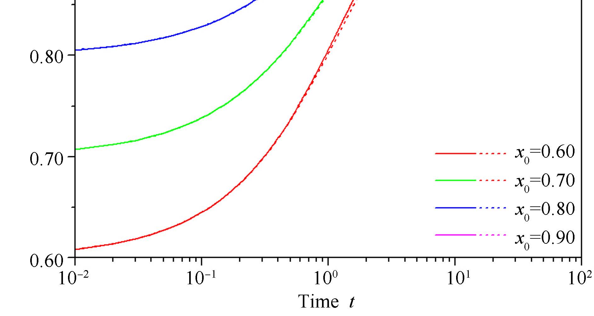
the solution equation (17) reduces to (8) at $\beta =1$, as it should. However, the solution to the FLM has not been published previously and in Fig. 1 we present a comparison of the analytic solution with the solution obtained from a numerical integration of the FLE. The numerical integration was performed with the help of Adams-Bashforth-Moulton predictor-corrector technique, developed by Diethelm et al.[18]. The two calculations differ by 2% at most and this deviation is discussed elsewhere[23].

|
Download:
|
| Fig. 1 The solid lines are the analytic solutions to the FLM and the dashed curves are from the numerical integration of the FLE. The four different sets of curves are for the initial conditions indicated. The time scale parameter is $\gamma=0.5$ and the Landau parameter is $\alpha=1.0$. The step of numerical integration is $h=10^{-3}$. | |
The rapidly decaying exponential function in the Landau model is replaced with the slowly decaying MLF in the FLM, since the MLF has the scale-free property in the asymptotic limit
| \begin{equation} \underset{\tau \rightarrow \infty }{\lim }E_{\beta }\left( -2k\gamma \tau^{\beta }\right) \propto \frac{1}{\tau ^{\beta }}. \label{asymptotic2} \end{equation} | (18) |
In the $\gamma \rightarrow 0$ limit of criticality the MLF can be replaced with the exponential:
| \begin{equation*} \underset{\gamma \rightarrow 0}{\lim }E_{\beta }\left( -2k\gamma \tau^{\beta }\right) \propto \exp \left( -2k\gamma \tau ^{\beta }\right) , \end{equation*} | (19) |
and (17) simplifies to
| \begin{equation} \underset{\gamma , \tau \rightarrow 0}{\lim }u\left( \tau \right) =\frac{u_{0}}{1+\alpha u_{0}\tau ^{\beta }}, \label{critical fractional} \end{equation} | (20) |
so that with memory and $0<\beta <1, $ the transition to turbulence is slower than in the memoryless case, since asymptotically $\tau >\tau ^{\beta }$ for $\beta <1$.
The solution given by (19) predicts that the energy of the turbulent flow field, at a point in space, asymptotically decays as an inverse power law in time. Numerical calculations of the Euler equations using the "t-model" in 2D and 3D yield inverse power-law decay with $\beta =1.84$[24]. The solution to the fractional Landau model must therefore be generalized to $1<\beta <2.$ This can be done by expressing the solution in terms of its initial value $u_{0}$, taking the initial time derivative $\overset{\cdot }{u}_{0}=0$ and noting that as $\gamma \rightarrow 0$ the critical slowing down maintains the asymptotic form $1/\tau ^{\beta }$, although now $\tau ^{\beta }>\tau $, asymptotically, since $\beta >1$. The decay of turbulent fluctuations is faster than in the memoryless case, but certainly much slower than the pre-critical exponential case.
Ⅳ. CONCLUSIONIn summary the spectral decomposition of the solution to a nonlinear dynamic equations can be generalized to fractional nonlinear rate equations and subsequently solved without approximation [21, 23]. In considering the Landau model for the transition to turbulence we used a phenomenological argument to motivate replacing the first-order with a fractional-order time derivative, but that need not be done. Stanislavsky[25] used subordination theory to develop a fractional Hamiltonian formalism, in which Hamilton's equations are given in terms of fractional derivatives. Memory is entailed by the dynamics of systems so described. He observed that space and time in these complex systems are not the continuous featureless processes first assumed by Newton[14], and turbulence certainly qualifies as being complex.
ACKNOWLEDGMENTThe authors would like to thank the U.S. Army Research Office for supporting this research.
| [1] | Arnold V I. Mathematical Methods of Classical Mechanics(Second Edition). New York: Springer-Verlag, 1989. |
| [2] | Lichtenberg A J, Lieberman M A. Regular and Stochastic Motion. New York: Springer-Verlag, 1983. |
| [3] | Koopman B O. Hamiltonian systems and transformation in Hilbert space. Proceedings of the National Academy of Sciences of the United States of America, 1931, 17: 315-318 |
| [4] | von Neumann J. Zur Operatorenmethode in der klassischen Mechanik. Annals of Mathematics, 1932, 33: 587-642 |
| [5] | von Neumann J. Züsatze zur Arbeit zur Operatorenmethode. Annals of Mathematics, 1932, 33: 789-791 |
| [6] | Kowalski K. Methods of Hilbert Spaces in the Theory of Nonlinear Dynamical Systems. Singapore: World Scientific, 1994. |
| [7] | Lindenberg K, West B J. The Nonequilibrium Statistical Mechanics of Open and Closed Systems. New York: Wiley-VCH, 1990. |
| [8] | Stiassnie M. On the application of fractional calculus for the formulation of viscoelastic models. Applied Mathematical Modelling, 1979, 3(4): 300-302 |
| [9] | Magin R L. Fractional calculus models of complex dynamics in biological tissues. Computers & Mathematics with Applications, 2010, 59(5): 1586-1593 |
| [10] | Henry B I, Langlands T A M, Wearne S L. Fractional cable models for spiny neuronal dendrites. Physical Review Letters, 2008, 100(12): 128103 |
| [11] | Garra R. Fractional-calculus model for temperature and pressure waves in fluid-saturated porous rocks. Physical Review E, 2011, 84(3): 036605 |
| [12] | Prajapati J C, Patel A D, Pathak K N, Shukla A K. Fractional calculus approach in the study of instability phenomenon in fluid dynamics. Palestine Journal of Mathematics, 2012, 1(2): 95-103 |
| [13] | West B J. Colloquium: fractional calculus view of complexity: a tutorial. Reviews of Modern Physics, 2014, 86(4): 1169-1186 |
| [14] | West B J. Fractional Calculus View of Complexity: Tomorrow's Science. New York: CRC Press, 2015. |
| [15] | Grigolini P, Rocco A, West B J. Fractional calculus as a macroscopic manifestation of randomness. Physical Review E, 1999, 59(3): 2603-2613 |
| [16] | Monin A S, Yaglom A M, Lumley J L. Statistical Fluid Mechanics. Vol. 1: Mechanics of Turbulence. Cambridge, MA: The MIT Press, 1971. |
| [17] | Landau L D, Lifshitz E M. Fluid Mechanics (Second Edition). Vol. 6. Course of Theoretical Physics. U.S.A.: Butterworth-Heinemann, 1987. |
| [18] | Diethelm K, Ford N J, Freed A D, Luchko Y. Algorithms for the fractional calculus: a selection of numerical methods. Computer Methods in Applied Mechanics and Engineering, 2005, 194(6-8): 743-773 |
| [19] | Cooper N G. Putting design into turbulence. 1663, Los Alamos Science & Technology Magazine. 2009. 10-15 |
| [20] | Podlubny I. Fractional Differential Equations. New York: Academic Press, 1999. |
| [21] | Svenkeson A, Glaz B, Stanton S, West B J. Spectral decomposition of nonlinear systems with memory. to be published |
| [22] | West B J, Bologna M, Grigolini P. Physics of Fractal Operators. New York: Springer, 2003. |
| [23] | Turalska M, West B J. A search for a spectral technique to solve nonlinear fractional differential equations. to be published |
| [24] | Hald O H, Stinis P. Optimal prediction and the rate of decay for solutions of the Euler equations in two and three dimensions. Proceedings of the National Academy of Sciences of the United States of America, 2007, 104: 6527-6532 |
| [25] | Stanislavsky A A. Hamiltonian formalism of fractional systems. The European Physical Journal B, 2006, 49(1): 93-101 |