 2016, Vol.3


2. State Key Laboratory of Management and Control for Complex Systems, Institute of Automation, Chinese Academy of Sciences, Beijing 100190, China
TRAFFIC control remains a hard problem for researchers and engineers, due to a number of difficulties. The major two are the modeling difficulty and the optimization difficulty.
First, transportation systems are usually distributed, hybrid and complex[1, 2, 3, 4, 5]. How to accurately and also conveniently describe the dynamics of transportation systems still leaves not fully solved. As pointed out in [5] and [6], most recent control systems aim to predict future states of transportation systems and make appropriate signal plans in advance. This requirement highlights the importance and hardness of transportation systems' modeling.
There are mainly two kinds of approaches to solve this difficulty[5]. One kind is the flow model based approaches, which formulate analytical models to describe the dynamics of macroscopic traffic flow measured at different locations. For example, cell transmission models (CTM) and its variations were frequently considered in reports due to its simplicity and effectiveness[7]. However, when traffic scenarios are complex, the modeling costs and errors need to be carefully considered.
The other kind is the simulation based approaches, which estimate/predict future traffic flow states using either artificial intelligence learning or simulations[8, 9, 10]. Artificial intelligence models learn and reproduce macroscopic traffic flow dynamics based on recorded traffic flow measurements. In contrast, simulations describe and reproduce the actions of individual microscopic traffic participators, which as a result provides flexible power to better describe macroscopic traffic flow dynamics. However, both artificial intelligence learning and simulation are time-consuming. The tuning of the control performance also becomes hard, since no theoretical analysis tool can be straightforwardly applied for these approaches.
Second, when traffic flow descriptions are established, how to determine the best signal plans becomes another problem. For flow model based approaches, we can use mathematical programming methods to solve the given objective functions (usually in terms of delay or queue length) with the explicitly formulated constraints derived from analytical models[7, 11, 12, 13].
Differently, for artificial intelligence learning and simulation based approaches, we will reverse the cause-effect based on the learned relationships between control actions and their effect on traffic flows. The try-and-test methods are then used to seek a (sub)optimal signal plan, based on the predicted or simulated effects of the assumed control actions. In literatures, heuristic optimization algorithms, such as genetic algorithms (GA)[14] were often applied to accelerate the seeking process. However, the converging speeds of such algorithms are still questionable in many cases.
In this paper, we focus on reinforcement learning approach for traffic signal timing problems[15, 16, 17, 18]. Reinforcement learning approach implicitly models the dynamics of complex systems by learning the control actions and the resulted changes of traffic flow. Meanwhile, it seeks the (sub)optimal signal plan from the learned input-output pairs.
The major difficulty of reinforcement learning for traffic signal timing lies in the exponentially expanding complexity of signal timing design with the number of the considered traffic flow states and control actions.
Recently, a new method is proposed to simultaneously solve the modeling and optimization problems of complex systems by using the so called deep Q network[19]. The deep Q networks indeed combine two hot tools: reinforcement learning[20] and deep learning[21, 22, 23]. Herein, deep learning uses multiple layers of artificial neural networks to learn the implicit maximum discounted future reward when we perform a special action given a special state.
In this paper, we examine the feasibility and effectiveness of this deep reinforcement learning method in building traffic signal timing plan. Although a few approaches have been proposed to approximate the maximum discounted future reward[16], our numerical tests show that deep networks provides a more convenient and powerful tool to reach this goal.
To give a more detailed explanation of our new designs, we will first present the new signal timing approach using deep learning in Section II; then in Section III, we provide some simulation results to show the effectiveness of the proposed new approach; finally, we conclude the paper in Section IV.
Ⅱ. Problem Presentation and The New Approach A. The Reinforcement Learning Traffic ControllerLet us define $s_t$ as the system states at time $t$, $a_t$ as the action at time $t$. $p$ denotes a policy, the rule how an action is chosen in each state. It characterizes a mapping from the state set $S$ to the action set $A$.
At each time step, the controller observes state $s_t $ and chooses an action $a_t$ to perform. The state of the system will be altered from $s_t$ to $s_{t+1}$ in the next time $t+1$, and a real-valued reward $r_t$ will be received. All the records $\left( {s_t , a_t , r_t , s_{t+1}} \right)$ will be stored into a replay memory to find the best policy that gives the highest reward.
We define the discounted future reward $R_t $ from time $t$ as
| \begin{equation} \label{eq1} R_t =\sum\limits_{i=t}^\infty {\gamma ^{i-t}r_i } =r_t +\gamma R_{t+1}, \end{equation} | (1) |
where $\gamma \in \left[{0, 1} \right]$ are the discount factor.
Suppose we always choose an action that maximizes the (discounted) future reward. Particularly, we define the so called Q-function $Q \left( {s_t , a_t } \right)$ that represents the maximum discounted future reward when we perform action $a_t$ in state $s_t$, and continue optimally from time $t$ onward. That is,
| \begin{equation} \label{eq2} p(s)=\mathop {\arg} \max \limits_a Q(s, a). \end{equation} | (2) |
Equation (2) has the property of the Bellman equation. So we can iteratively approximate the Q-function using
| \begin{equation} \label{eq3} Q(s, a)=r+\gamma \mathop {\max }\limits_{{a'}} Q({s'}, {a'}). \end{equation} | (3) |
This form can be explained as the maximum future reward for the current state and action is the current reward plus the maximum future reward for the next state.
If $Q \left( {s_t , a_t } \right)$ is known, we can directly solve (3) to find the optimal policy. However, $Q \left( {s_t , a_t } \right)$ is usually unknown. So, we need to estimate $Q \left( {s_t , a_t } \right)$ in the learning process. In early stages of learning, $Q \left( {s_t , a_t } \right)$ may be completely wrong. However, the estimation gets more and more accurate with every iteration of updating.
For traffic signal timing problems for intersections, traffic sensors measure the states (speed, queueing length, etc.) of traffic flows. We consider all these measures as system states. The actions here are giving rights of way for each specified traffic stream. So, after one action $a_t $ is performed, traffic states will be changed from $s_t $ to $s_{t+1}$. We also calculate a reward $r_t $ (the performance like traffic delay and queue length) after each action.
B. The Deep Reinforcement-Learning Traffic ControllerIn conventional approaches, the Q-function is implemented using a table or a function approximator[17, 18]. However, the state spaces of traffic signal timing problems is so huge that we can hardly solve the formulated reinforcement learning problem within a finite time with a table based Q learning method; and the traditional function approximator based Q learning method can hardly capture dynamics of traffic flow.
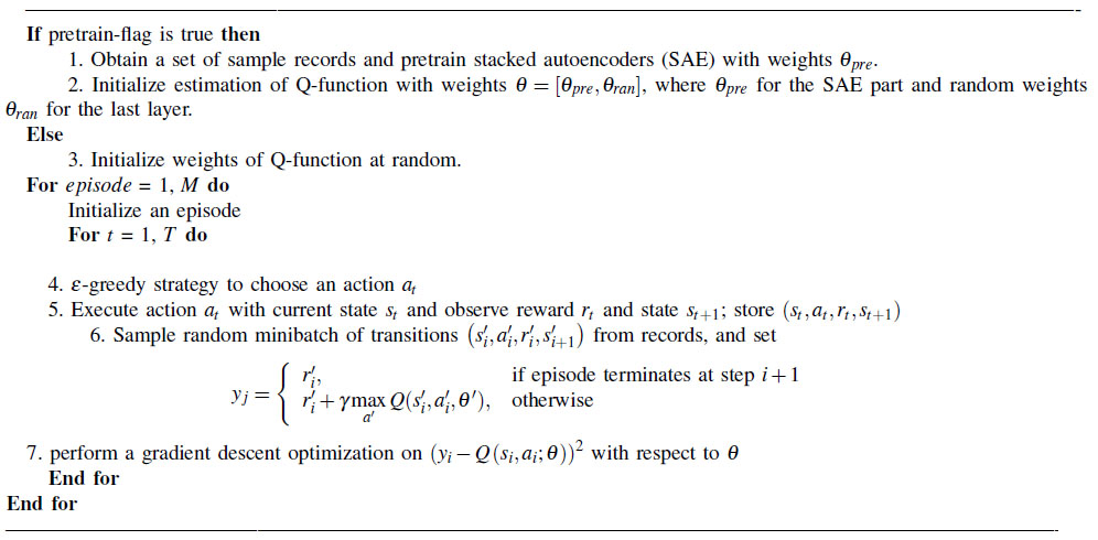
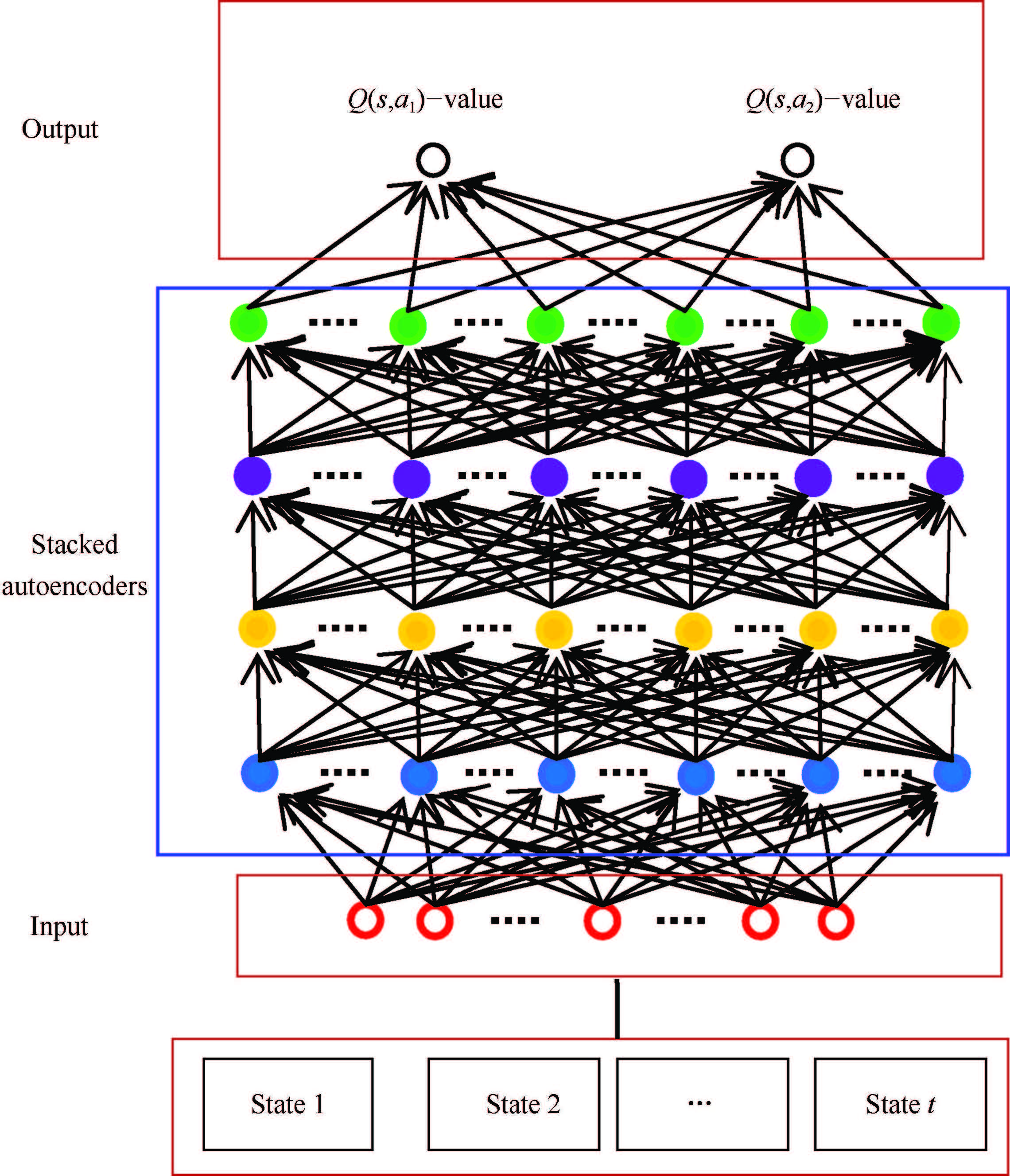
In contrast, we use the deep stacked autoencoders (SAE) neural network[23, 24] to estimate the Q-function here. This neural network takes the state as input and outputs the Q-value for each possible action. Fig. 1 gives an illustration of its structure. As its name indicates, the SAE neural network contains multiple hidden layers of autoencoders where the outputs of each layer is wired to the inputs of the successive layer.

|
Download:
|
| Fig. 1 The deep SAE neural network for approximating Q function. | |
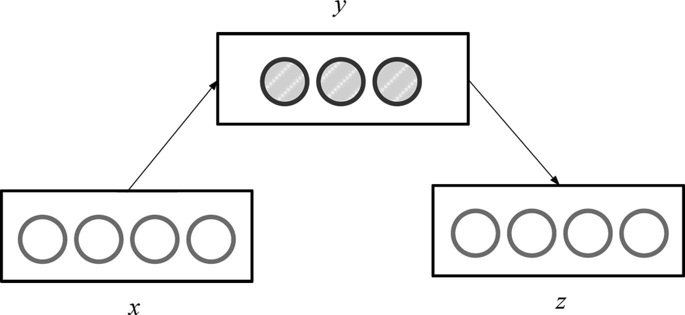
Autoencoders are building blocks of creating the deep SAE neural network. An autoencoder is a neural network that sets the target output to be equal to the input. Fig. 2 gives an illustration of an autoencoder, which has three layers: one input layer, one hidden layer, and one output layer.

|
Download:
|
| Fig. 2 An autoencoder. | |
Given an input $x$, an autoencoder first encodes the input $x$ to a hidden representation $y\left( x \right)$ based on (4), and then decodes the representation $y\left( x \right)$ back into a reconstruction $z\left( x \right)$ computed as in (5). The objective of an autoencoder is to learn a mapping that produces $z\left( x \right)\approx x$.
| \begin{equation} y(x)=h(W_1 x+b), \end{equation} | (4) |
| \begin{equation} z(x)=h'(W_2 y (x)+c), \end{equation} | (5) |
where $W_1 $ and $W_2 $ are weight matrices, $b$ and $c$ are bias vectors.
The model parameters $\theta _{ae}$ of an auctoencoder can be obtained by minimizing the reconstruction error $L\left( {X, Z}\right)$:
| \begin{equation} \label{eq6} \begin{array}{c} \theta_{ae} =\mathop {\arg} \min\limits_{\theta _{ae} } L\left( {X, Z} \right)~~~~~~~~~~~~~~ \\ ~~~~~~~~~~~~~~~=\mathop {\arg} \min\limits_{\theta _{ae} } \frac{1}{2}\sum{\left\| {x-z\left( x \right)} \right\|^2} +\beta \sum\limits_{j=1}^{H_D } {\mbox{KL}\left( {\rho \vert \vert \hat {\rho }_j } \right), } \\ \end{array} \end{equation} | (6) |
where $\beta $ is the weight of the sparsity penalty term, $H_D $ is the number of hidden units, $\rho $ is a sparsity parameter, and $\hat {\rho }_j =\frac{1}{N}\sum\nolimits_{i=1}^N {y_j \left( {x^{(i)}} \right)} $is the average activation of the hidden unit $j$ over the training set.
The Kullback-Leibler (KL) divergence $\mbox{KL}\left( {\rho \vert \vert \hat {\rho }_j } \right)$ is defined as
| \[ \mbox{KL}\left( {\rho \vert \vert \hat {\rho }_j } \right)=\rho \log \frac{\rho }{\hat {\rho }_j }+\left( {1-\rho } \right)\log \frac{1-\rho }{1-\hat {\rho }_j }. \] |
We take greedy layerwise approach to train each layer in turn, so that autoencoders can be ``stacked" in a greedy layerwise fashion for pretraining (initializing) the weights of a deep network. The obtained approximation of Q function is written as $Q\left( {s_t , a_t , \theta } \right)$, with $\theta $ characterizes the values of weights and other parameters of SAE network.
During Q-learning, this deep SAE is trained by minimizing the following simple loss function over samples of experience till time $t$:
| \begin{equation} \label{eq7} L(\theta )=\left[{\underbrace {r+\gamma \mathop {\max }\limits_{{a}'} Q({s}', {a}', {\theta }')}_{\mbox{target}}-\underbrace {Q({s}', {a}', \theta )}_{\mbox{prediction}}} \right]^2, \end{equation} | (7) |
where a record $\left( {{s}'_t , {a}'_t , {r}'_t , {s}'_{t+1} } \right)$ is drawn randomly from the replay memory.
Once we had set up a policy after we observe a certain number of records, we will face the explore-exploit dilemma: Should we exploit the current working policy or explore other (possibly better) policies. To solve this problem, we apply the $\varepsilon $-greedy strategy. That is, with probability $\varepsilon$ we select a random action and with probability $1-\varepsilon$ to follow the current policy.
In summary, the detailed learning algorithm is shown in Algorithm 1.
|
|
Algorithm 1 The deep reinforcement learning algorithm for traffic signal control |
In pretraining procedure, we take greedy layerwise approach to train each layer in turn, so that autoencoders can be ``stacked" in a greedy layerwise fashion for pretraining (initializing) the weights of a deep network. The obtained approximation of Q function is written as $Q\left( {s_t, a_t, \theta } \right)$, with $\theta $ characterizes the values of weights and other parameters of SAE network.
During Q-learning, this deep SAE is trained by minimizing the following simple loss function over samples of experience till time $t$.
Ⅲ. Simulation ResultsTo compare the proposed deep reinforcement learning traffic controller and the conventional traffic controller, we design the following cases.
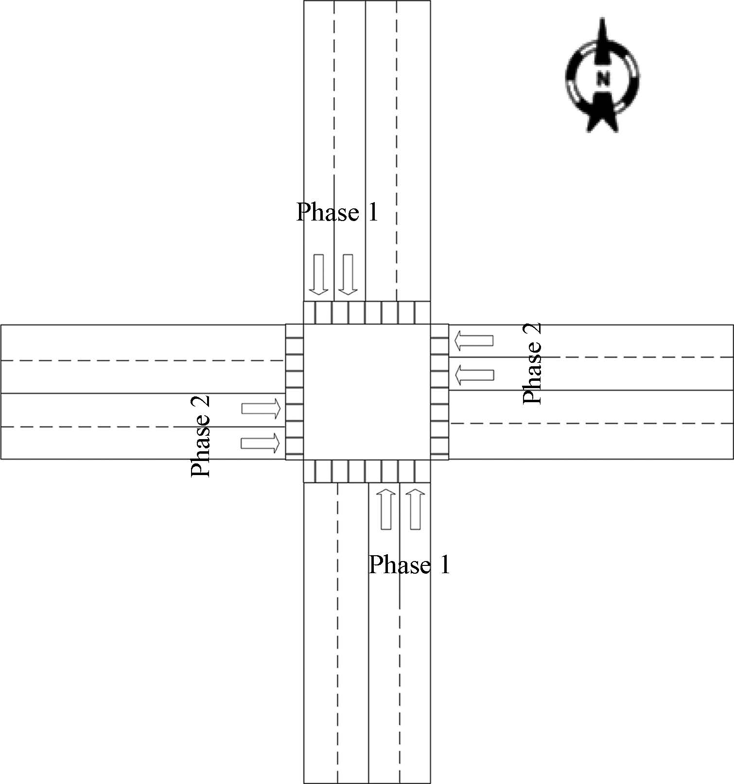
The geometry of the studied crossing is shown in Fig. 3. Each branch of the intersection has four lanes (two lanes for coming vehicles and two for leaving ones). In other words, there are 8 incoming lanes connected to this intersection. No left-turn, right-turn or U-turn is allowed.

|
Download:
|
| Fig. 3 The geometry of the simulated intersection. | |
Suppose there are two phases here: one phase allows vehicles running either north-to-south or south-to-north to enter the intersection, the other phase allows vehicles running either east-to-west or west-to-east to enter the intersection. We assume that there is no red-clearance time here, so one phase appears immediately after another phase. The minimum green time is 15 s for both two phases.
We measure the queueing lengths of the 8 incoming lanes per 5 s, and the values are denoted $q_t^{e-w, 1} $, $q_t^{e-w, 2} $, $q_t^{w-e, 1} $, $q_t^{w-e, 2} $, $q_t^{n-s, 1} $, $q_t^{n-s, 2} $, $q_t^{s-n, 1} $, $q_t^{s-n, 2} $ at sampling time $t$. We take the measured queueing lengths during the last four samples as the state of the system at time $t$. There are only two actions: remain the current phase, change to the other phase (it must be pointed out that the second action might be forbidden sometimes if the current phase has not yet lasted for 15 s).
We use PARAMICS to simulate the traffic flow dynamics with given traffic states and actions. The reward is defined as the absolute value of the difference between north-south/south-north direction and east-west/west-east direction, i.e.
| \begin{equation} \label{eq5} r_t =\left| {\mathop {\max }\limits_{i=1, 2} \left\{ {q_t^{e-w, i}, q_t^{w-e, i} } \right\}-\mathop {\max }\limits_{i=1, 2} \left\{ {q_t^{s-n, i}, q_t^{s-n, i} } \right\}} \right|. \end{equation} | (8) |
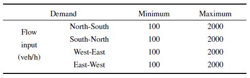
For both conventional reinforcement learning and the new deep reinforcement learning traffic controller, we pretrain the controller with randomly generated traffic demands shown in Table I. The minimum traffic demand for each approach is 100 veh/h and the maximum is 2000 veh/h.
|
|
Table Ⅰ THE TRAFFIC DEMANDS USED FOR PRETRAINING |
In both pretraining and testing cases, we set $\gamma =0.1$ and let $\varepsilon $ vary as
| \begin{equation} \varepsilon =\max \left\{ 0.001, 1-\frac{t}{500} \right\}. \end{equation} | (9) |
It should be pointed out that we had tested other settings of $\gamma $ and $\varepsilon $. Results indicate that the performance difference between conventional and new deep reinforcement learning methods remained unchanged.
For the new deep reinforcement learning traffic controller, we choose a four-layer SAE neural network which has two hidden layers. There are 32 neurons in the input layer, since we input the 8 queueing length values during the last four sampling intervals. There are just 2 neurons in the output layer, since we only have two actions. There are 16 and 4 neurons in the hidden two layers, respectively. The activation function for hidden layers is the sigmoid function.
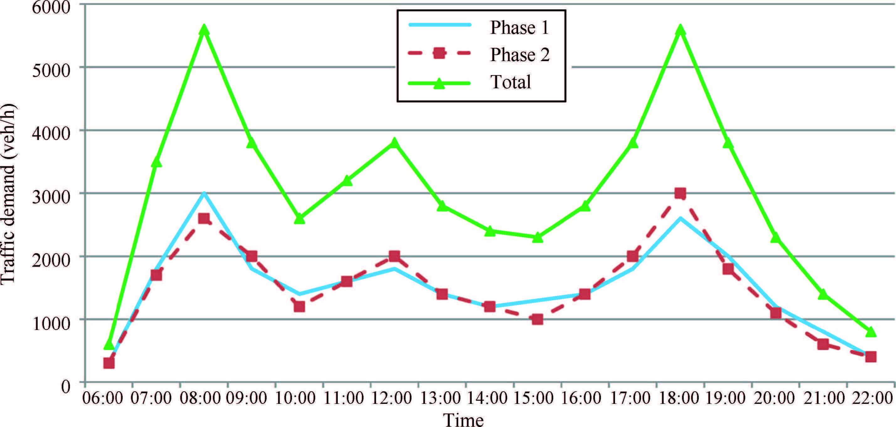
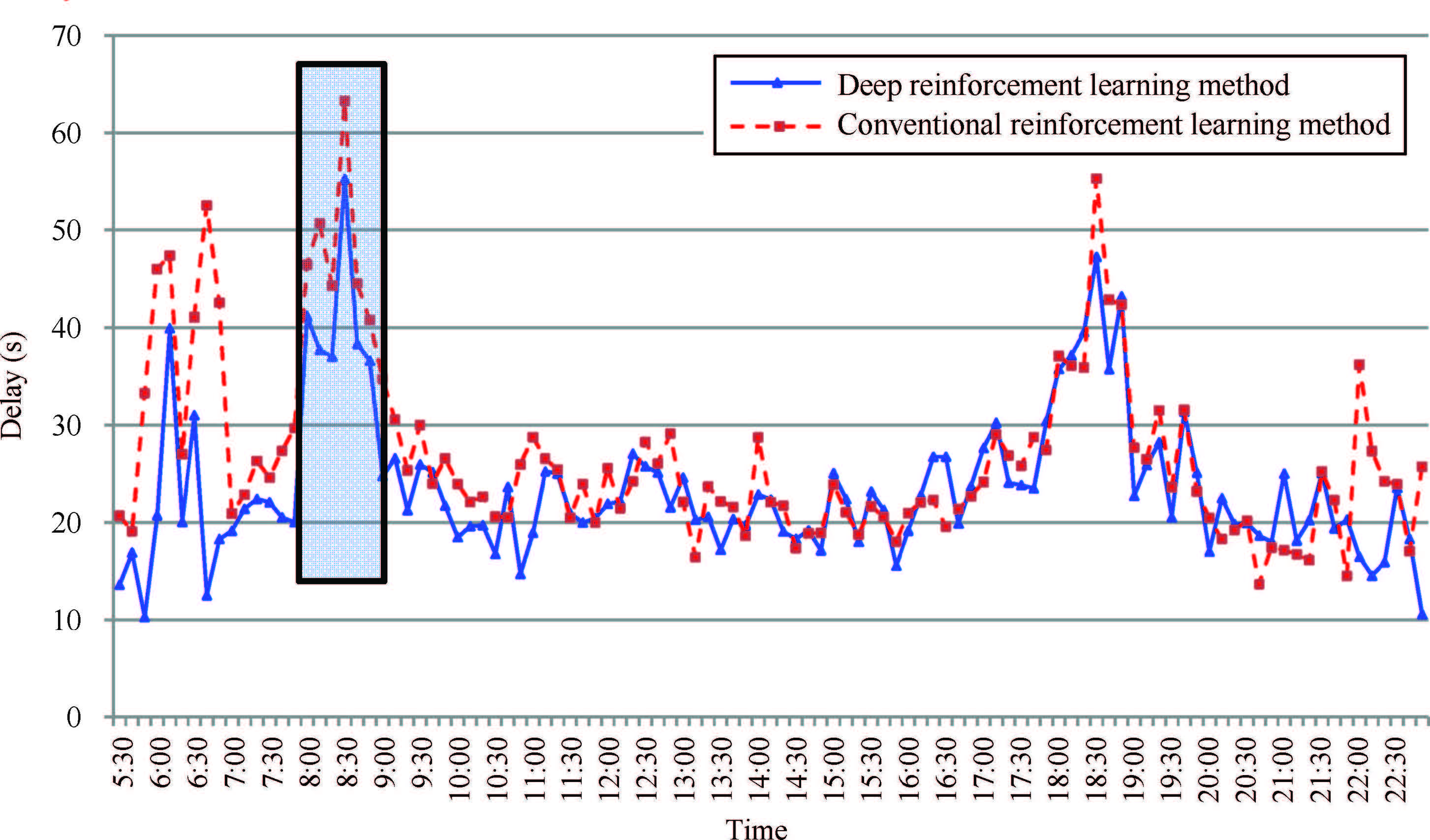
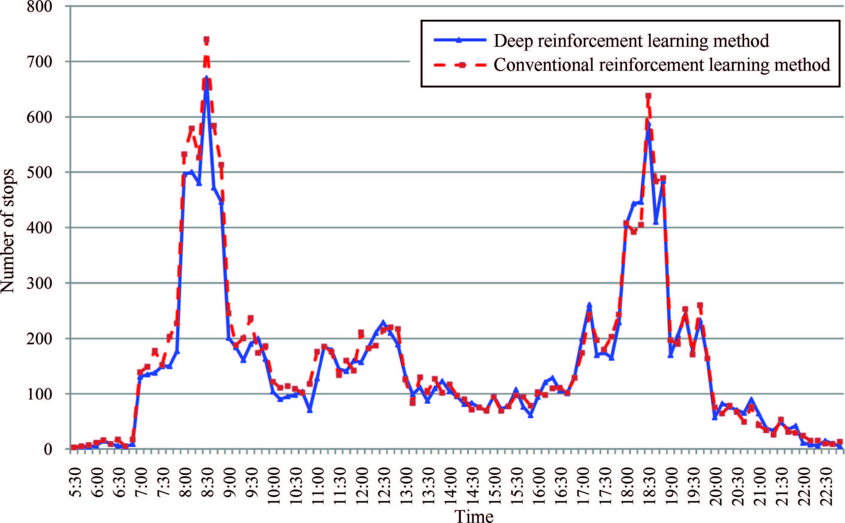
Fig. 4 gives the traffic demands used for testing. Fig. 5 and Fig. 6 give the comparison between the delay and the number of stops queueing lengths observed when deep reinforcement learning method and conventional ordinary reinforcement learning method are used, respectively.

|
Download:
|
| Fig. 4 The traffic demands used for testing. | |

|
Download:
|
| Fig. 5 The delay observed when deep reinforcement learning method and conventional reinforcement learning method are used. | |

|
Download:
|
| Fig. 6 The number of stops observed when deep reinforcement learning method and conventional reinforcement learning method are used. | |
Considering the uncertainty of simulation with randomness, we further compare the mean values of the obtained delay and the number of fully stopped vehicles of two reinforcement learning traffic controller during 20 times of simulations.
We find that the average delay can be reduced about 14 ${\%}$ if the deep reinforcement learning method is used instead of conventional ordinary reinforcement learning method. In morning peak hours, a vehicle may spend about 13 s less to pass the studied intersection.
Moreover, the number of fully stopped vehicles is reduced by 1020 vehicles when the deep reinforcement learning method is applied. Particularly, the number of fully stopped vehicles is reduced by 410 vehicles in morning peak hours.
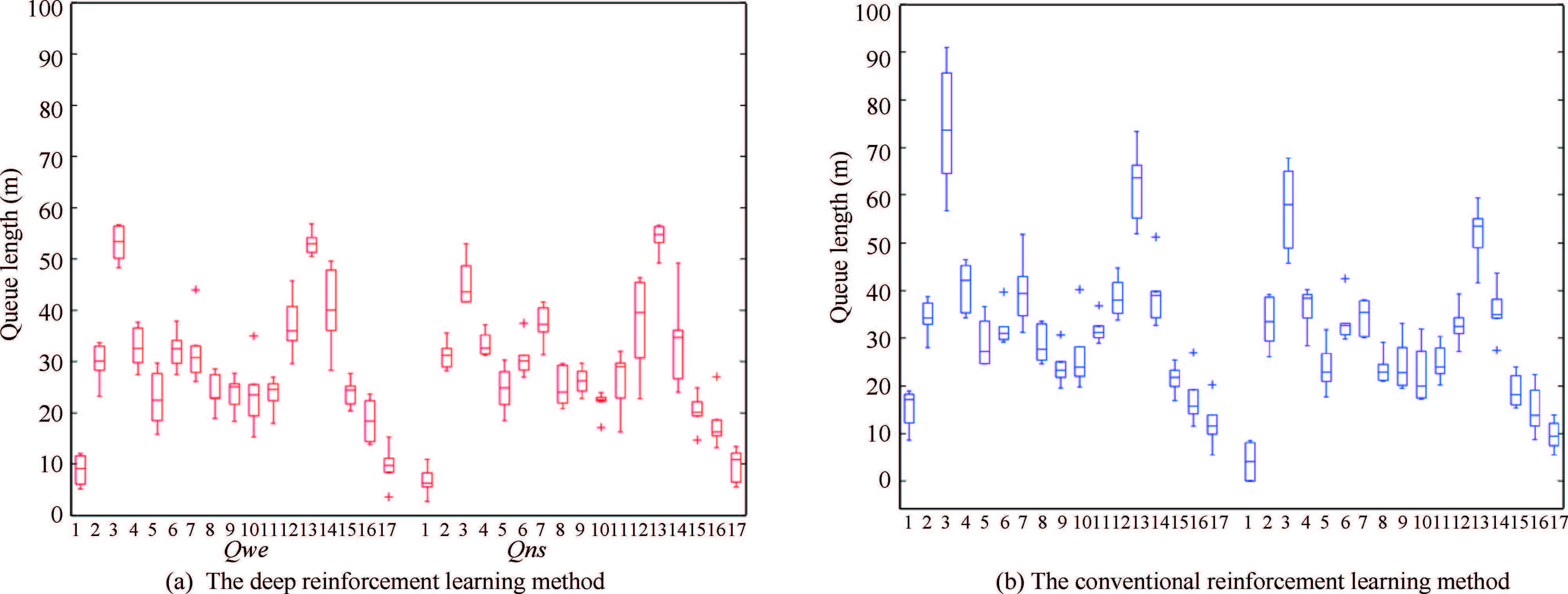
Let $Qns$ denotes the queue length in the N-S direction, $Qwe$ denote the queue length in the W-E direction Fig. 7 shows the box plot of queue lengths in the N-S and W-E directions generated by the conventional reinforcement learning method and the deep reinforcement learning method proposed in this paper. Clearly, the queue length generated by the deep reinforcement learning method is less than that generated by the conventional reinforcement learning method.

|
Download:
|
| Fig. 7 Box plots of queue lengths of the deep reinforcement learning method and the conventional reinforcement learning method in the test scenario. | |
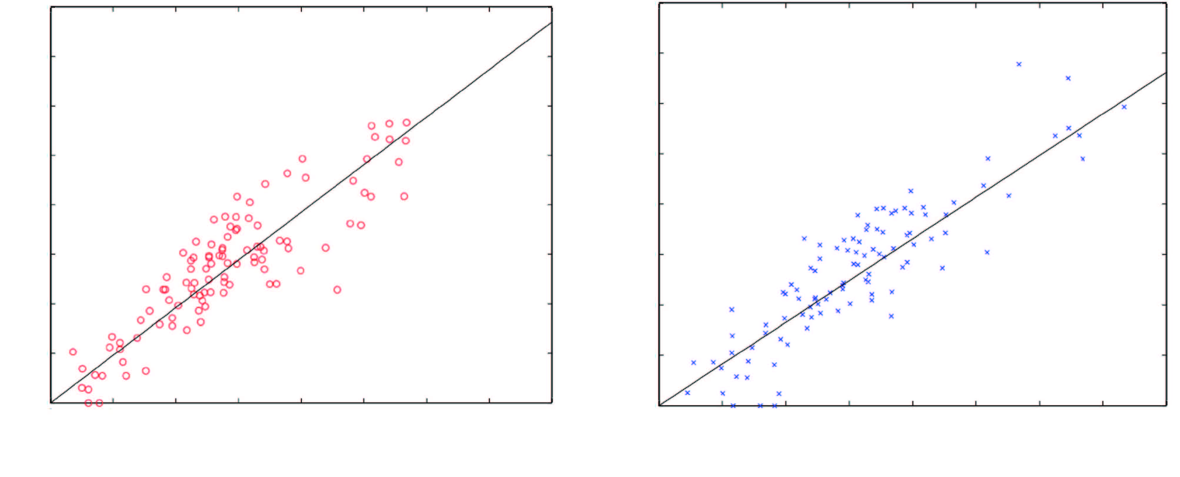
Fig. 8 shows the scatter plots of queue states in the test scenario. We assess the queue balance using the linear regression $R^{2}$ of the queue states. As indicated in [25] and [26], a larger $R^{2}$ value indicates more balanced queues. We can observe that the conventional reinforcement learning method and the deep reinforcement learning method proposed in this paper can have similar effects on producing balanced queues in the N-S and W-E directions. However, as indicated in Fig. 5, the deep reinforcement learning control can maintain less queue length than the conventional reinforcement learning method. Nevertheless, the conventional reinforcement learning method sometimes generates extremely long queue lengths.

|
Download:
|
| Fig. 8 Scatter plots of queue states of the deep reinforcement learning method and the conventional reinforcement learning method in the test scenario. | |
Reinforcement learning had gained increasing interests in traffic control field. Different from traffic flow model based control strategy, it simultaneously learn the dynamics of traffic systems and the optimal control plan by implicitly modeling the control actions and the change of system states.
In this paper, we apply the deep reinforcement learning method[19] developed recently and show that it notably outperforms conventional approaches in finding a better signal timing plan. We believe the combination of such deep knowledge representation, deep reinforcement learning method and parallel intelligent transportation systems[8, 9, 10, 27, 28, 29, 30, 31, 32] may have great potential to change the development course of next-generation ITS.
| [1] | Mirchandani P, Head L. A real-time traffic signal control system: architecture, algorithms, and analysis. Transportation Research, Part C: Emerging Technologies, 2001, 9(6): 415-432 |
| [2] | Papageorgiou M, Diakaki C, Dinopoulou V, Kotsialos A, Wang Y B. Review of road traffic control strategies. Proceedings of the IEEE, 2003, 91(12): 2043-2067 |
| [3] | Mirchandani P, Wang F Y. RHODES to intelligent transportation systems. IEEE Intelligent Systems, 2005, 20(1): 10-15 |
| [4] | Chen B, Cheng H H. A review of the applications of agent technology in traffic and transportation systems. IEEE Transactions on Intelligent Transportation Systems, 2010, 11(2): 485-497 |
| [5] | Li L, Wen D, Yao D Y. A survey of traffic control with vehicular communications. IEEE Transactions on Intelligent Transportation Systems, 2014, 15(1): 425-432 |
| [6] | Bellemans T, De Schutter B, De Moor B. Model predictive control for ramp metering of motorway traffic: a case study. Control Engineering Practice, 2006, 14(7): 757-767 |
| [7] | Timotheou S, Panayiotou C G, Polycarpou M M. Distributed traffic signal control using the cell transmission model via the alternating direction method of multipliers. IEEE Transactions on Intelligent Transportation Systems, 2015, 16(2): 919-933 |
| [8] | Wang F Y. Parallel control and management for intelligent transportation systems: concepts, architectures, and applications. IEEE Transactions on Intelligent Transportation Systems, 2010, 11(3): 630-638 |
| [9] | Wang F Y. Agent-based control for networked traffic management systems. IEEE Intelligent Systems, 2005, 20(5): 92-96 |
| [10] | Li L, Wen D. Parallel systems for traffic control: a rethinking. IEEE Transactions on Intelligent Transportation Systems, 2015, 17(4): 1179-1182 |
| [11] | Liu H C, Han K, Gayah V V, Friesz T L, Yao T. Data-driven linear decision rule approach for distributionally robust optimization of on-line signal control. Transportation Research, Part C: Emerging Technologies, 2015, 59: 260-277 |
| [12] | Yang I, Jayakrishnan R. Real-time network-wide traffic signal optimization considering long-term green ratios based on expected route flows. Transportation Research, Part C: Emerging Technologies, 2015, 60: 241-257 |
| [13] | Rinaldi M, Tampre C M J. An extended coordinate descent method for distributed anticipatory network traffic control. Transportation Research, Part B: Methodological, 2015, 80: 107-131 |
| [14] | Sánchez-Medina J J, Galán-Moreno M J, Rubio-Royo E. Traffic signal optimization in La Almozara district in Saragossa under congestion conditions, using genetic algorithms, traffic microsimulation, and cluster computing. IEEE Transactions on Intelligent Transportation Systems, 2010, 11(1): 132-141 |
| [15] | Bingham E. Reinforcement learning in neurofuzzy traffic signal control. European Journal of Operational Research, 2001, 131: 232-241 |
| [16] | Prashanth L A, Bhatnagar S. Reinforcement learning with function approximation for traffic signal control. IEEE Transactions on Intelligent Transportation Systems, 2011, 12(2): 412-421 |
| [17] | El-Tantawy S, Abdulhai B, Abdelgawad H. Multiagent reinforcement learning for integrated network of adaptive traffic signal controllers (MARLIN-ATSC): methodology and large-scale application on downtown Toronto. IEEE Transactions on Intelligent Transportation Systems, 2013, 14(3): 1140-1150 |
| [18] | Ozan C, Baskan O, Haldenbilen S, Ceylan H. A modified reinforcement learning algorithm for solving coordinated signalized networks. Transportation Research, Part C: Emerging Technologies, 2015, 54: 40-55 |
| [19] | Mnih V, Kavukcuoglu K, Silver D, Rusu A A, Veness A, Bellemare M G, Graves A, Riedmiller M, Fidjeland A K, Ostrovski G, Petersen S, Beattie C, Sadik A, Antonoglou I, King H, Kumaran D, Wierstra D, Legg S, Hassabis D. Human-level control through deep reinforcement learning. Nature, 2015, 518(7540): 529-533 |
| [20] | Sutton R, Barto A. Reinforcement Learning: An Introduction. Cambridge, MA: MIT Press, 1998. |
| [21] | Hinton G E, Salakhutdinov R R. Reducing the dimensionality of data with neural networks. Science, 2006, 313(5786): 504-507 |
| [22] | Bengio y. Learning deep architectures for AI. Foundations and Trends in Machine Learning, 2009, 2(1): 1-127 |
| [23] | Lange S, Riedmiller M. Deep auto-encoder neural networks in reinforcement learning. In: Proceedings of the 2010 International Joint Conference on Neural Networks (IJCNN). Barcelona: IEEE, 2010. 1-8 |
| [24] | Abtahi F, Fasel I. Deep Belief Nets as function approximators for reinforcement learning. In: Proceedings of Workshops at the 25th AAAI Conference on Artificial Intelligence. Frankfurt, Germany: AIAA, 2011. |
| [25] | Lin W H, Lo H K, Xiao L. A quasi-dynamic robust control scheme for signalized intersections. Journal of Intelligent Transportation Systems: Technology, Planning, and Operations, 2011, 15(4): 223-233 |
| [26] | Tong Y, Zhao L, Li L, Zhang Y. Stochastic programming model for oversaturated intersection signal timing. Transportation Research, Part C: Emerging Technologies, 2015, 58: 474-486 |
| [27] | Wang F Y. Building knowledge structure in neural nets using fuzzy logic. in Robotics and Manufacturing: Recent Trends in Research Education and Applications, edited by M. Jamshidi, New York, NY, ASME (American Society of Mechanical Engineers) Press, 1992. |
| [28] | Wang F Y, Kim H M. Implementing adaptive fuzzy logic controllers with neural networks: a design paradigm. Journal of Intelligent & Fuzzy Systems, 1995, 3(2): 165-180 |
| [29] | Chen C, Wang F Y. A self-organizing neuro-fuzzy network based on first order effect sensitivity analysis. Neurocomputing, 2013, 118: 21-32 |
| [30] | Wang F Y. Toward a Revolution in transportation Operations: AI for Complex Systems. IEEE Intelligent Systems, 2008, 23(6): 8-13 |
| [31] | Wang F Y. Parallel system methods for management and control of complex systems. Control and Decision, 2004, 19(5): 485-489 (in Chinese) |
| [32] | Wang F Y. Parallel control: a method for data-driven and computational control. Acta Automatica Sinica, 2013, 39(4): 293-302 (in Chinese) |