 2016, Vol.3


PARALLEL machine scheduling problem (PMSP)[1] is a typical combinatorial optimization problem existing in many manufacturing systems[2, 3, 4]. According to the characteristic of machines, PMSP can be classified into three types: identical PMSP[5], where each job has an identical processing time on every machine; uniform PMSP[6], where the processing time of a job is inversely proportional to the processing speed of a machine; and unrelated PMSP (UPMSP)[7], where the processing times of a job on different machines are unrelated. Identical PMSP and uniform PMSP can be regarded as the special cases of UPMSP. As a complex scheduling problem, PMSP is NP-hard even in a two-machine case[8]. Therefore, it is important to study PMSP and to develop effective solution algorithms, especially for the most general one, UPMSP.
In the literature about the UPMSP, it is common to assume that there is no additional time between any two processing operations[7]. However, setup times widely exist in practice when preparing machines for the coming jobs[9]. Setup times are relevant to the job sequences on machines. During recent years, the UPMSP with sequence-dependent setup times (UPMSP-SDST) has been a focus in the area of PMSP. According to the reported research work before 2008, a brief review of the UPMSP-SDST was presented in [10]. Here, we focus on the typical literature after 2008.
To minimize the makespan of the UPMSP-SDST, Behnamian et al.[11] presented a hybrid algorithm based on ant colony optimization (ACO), simulated annealing (SA), and variable neighborhood search (VNS). The population was initialized by ACO and evolved by SA and VNS. Chang and Chen[12] presented a set of dominance properties as necessary conditions for inter- and intra-machine switching of job sequencing orders in a schedule. Besides, they proposed a genetic algorithm (GA) by integrating these dominance properties. Vallada and Ruiz[10] proposed a GA with a fast local search and a local-search-enhanced crossover operator. They also developed sets of benchmark instances to test the performances of algorithms in solving the UPMSP-SDST. It was shown that the proposed GA outperformed other evaluated methods in solving those benchmark instances. Besides, Fleszar et al.[13] hybridized the variable neighborhood descent (VND) with mathematical programming. Lin and Ying[14] presented a hybrid artificial bee colony algorithm. Yilmaz et al.[15] developed a GA with local search. Arnaout et al.[16] proposed an ACO and then enhanced the ACO by using a pheromone re-initialization method. Avalos-Rosales et al.[17] proposed a metaheuristic algorithm based on the multi-start algorithm and VND.
Considering the additional due-date constraints, some work aimed at minimizing the total tardiness of jobs. Chen[18] presented a hybrid heuristic based on the modified apparent-tardiness-cost-with-setup procedure, SA method, and improvement procedures. Lin et al.[19] presented an iterated greedy (IG) heuristic, which was shown to be more effective and efficient than the state-of-the-art algorithms.
To minimize the total completion time of all jobs, Hsu et al.[20] showed that there existed a polynomial time method for the problem with the past-sequence-dependent setup time and learning effects on machines. Then, they derived similar conclusions when minimizing the total absolute deviation of job completion times and the total load on all machines[21]. By supposing that a machine had a production availability, Joo and Kim[22] proposed a hybrid GA with three dispatching rules to minimize the total completion time.
For other objectives, Chen and Chen[23] developed several hybrid metaheuristics by integrating VND approach and tabu search to minimize the weighted number of tardy jobs. Lin and Ying[4] proposed a multi-point multi-objective SA algorithm to simultaneously minimize makespan, total weighted completion time, and total weighted tardiness.
As a population-based evolutionary algorithm, estimation of distribution algorithm (EDA) employs a probability model for optimization[24]. By sampling a promising area of the search space to generate new solutions, the EDA has a strong ability of global exploration. Due to its merits, the EDA has already been successfully applied to solve a variety of academic and engineering optimization problems[25]. However, to the best of our knowledge, it has never been applied to the UPMSP-SDST. Meanwhile, the EDA often shows good global exploration capability while its exploitation capability is relatively weak. Therefore, it motivates us to propose a hybrid EDA with the iterated greedy search[26] and especially some problem-specific properties, named EDA-IG, to balance the global exploration and the local exploitation for the UPMSP-SDST with makespan criterion. To be specific, some properties for judging the effectiveness of neighborhood search operators are analyzed to avoid invalid search operators. Based on neighbor relations of the jobs, a probability model is built to generate new solutions for global exploration. In addition, two types of deconstruction and reconstruction are designed to develop an IG search for local exploitation. With 1640 benchmark instances, numerical tests are carried out to show the effectiveness of the proposed EDA-IG and the properties.
The remainder of the paper is organized as follows: First, the UPMSP-SDST is briefly described in Section Ⅱ. Then, after analyzing the properties of the neighborhood search operators in Section Ⅲ, the EDA-IG for solving the UPMSP-SDST is presented in Section IV. In Section V, the influence of parameter setting is investigated and numerical results are provided. Finally the paper is ended with some conclusions and future work in Section VI.
Ⅱ. Problem Description A. Notation$n$: the number of jobs to be processed;
$m$: the number of machines;
$J_{i}$: the $i$-th job;
$M_{k}$: the $k$-th machine;
Cmax: the maximum completion time of jobs, i.e., makespan;
$C_{i}$: the completion time of $J_{i}$;
$P_{i,k}$: the processing time of $J_{i}$ on $M_{k}$;
$ST_{i,j,k}$: the setup time of processing $J_{j}$ right after $J_{i}$ on $M_{k}$;
$ST_{0,j,k}$: the setup time of processing $J_{j}$ first on $M_{k}$;
$X_{i,j,k}$: a binary variable that is equal to 1 if $J_{j}$ is right after $J_{i}$ on $M_{k}$,0 otherwise;
$X_{0,j,k}$: a binary variable that is equal to 1 if $J_{j}$ is the first one on $M_{k}$,0 otherwise;
$X_{j,0,k}$: a binary variable that is equal to 1 if $J_{j}$ is the last one on $M_{k}$,0 otherwise;
$V$: a very large constant;
$R_{k}$: the release (completion) time of $M_{k}$;
$N_{k}$: the total number of jobs on $M_{k}$;
$P_{[j],k}$: the processing time of the $j$-th job on $M_{k}$;
$ST_{[i],[j],k}$: the setup time of processing the $j$-th job right after the $i$-th one on $M_{k}$;
$AP_{i,j,k}$: the total needed (setup and processing) time for the $j$-th job right after the $i$-th one on $M_{k}$;
$ST_{[0],[1],k}$: the setup time of processing the first job on $M_{k}$;
$AP_{0,1,k}$: the total needed (setup and processing) time for the first job on $M_{k}$.
B. Mathematical ModelThe UPMSP-SDST with makespan criterion can be described as follows: There are $n$ jobs to be processed by $m$ machines. Each job has only one operation, which can be executed on any machine. Setup time is needed before processing a job. Setup time is job-sequence-dependent and machine-dependent. The objective is to determine the job processing sequences on all the machines to minimize the maximum completion time of all jobs. Usually, it assumes that: All the jobs and machines are available at the initial time; and each machine can process only one job, and each job can be processed on only one machine at a time; and once an operation starts, it cannot be interrupted before its completion. Mathematically, the UPMSP-SDST with makespan criterion can be formulated as follows[27]:
| \begin{equation} \min C_{\max}=\max\{C_{i}|i=1,2,\dots,n\}, \end{equation} | (1) |
Subject to:
| \begin{equation} \sum\limits_{i=0 \atop i \not= j}^{n}\sum\limits_{k=1}^{m} X_{i,j,k}=1,\,\forall j=1,2,\dots,n, \end{equation} | (2) |
| \begin{gather} \sum\limits_{i=0 \atop i \not= h}^{n} X_{i,h,k}-\sum\limits_{j=0 \atop j \not= h}^{n} X_{h,j,k}=0,\notag \\ \forall h=1,2,\dots,n; \forall k=1,2,\dots,m, \end{gather} | (3) |
| \begin{gather} C_{j}\ge C_{i}+\sum\limits_{k=1}^{m} X_{i,j,k}(ST_{i,j,k}+P_{j,k})+V(\sum\limits_{k=1}^{m} X_{i,j,k}-1),\notag \\ \forall i=0,1,\dots,n; \forall j=1,2,\dots,n, \end{gather} | (4) |
| \begin{equation} \sum\limits_{j=0}^{n} X_{0,j,k}=1,\,\forall k=1,2,\dots,m, \end{equation} | (5) |
| \begin{equation} X_{i,j,k} \in \{0,1\},\forall i,j=0,1,\dots,n;\forall k=1,2,\dots,m, \end{equation} | (6) |
| \begin{equation} C_{0}=0, \end{equation} | (7) |
| \begin{equation} C_{j}\ge 0,\forall j=1,\dots,n. \end{equation} | (8) |
Equation (1) is the objective function. Equation (2) ensures that every job should be processed only once. Equation (3) implies that each job has a predecessor and a successor. Note that, a dummy job $J_0$ is used to present the first job on a machine. Equation (4) ensures that the processing of a job should be started after the completion of its predecessor. Equation (5) ensures that each machine has only one dummy job. Equation (6) defines the binary variables. Equation (7) implies that the completion time of a dummy job is zero. Equation (8) ensures that the completion time of a regular job is non-negative.
Ⅲ. Properties of Neighborhood Search Operators
For shop scheduling problems, some typical neighborhood search operators are often used to find better solutions. Regarding the UPMSP-SDST, five operators are usually employed, including three inter-machine operators and two intra-machine operators.
A. Typical Operators for UPMSP-SDSTThe inter-machine operators are as follows (Let $j > i$ without loss of generality):
1) SWS($i$,$j$,$k$): Swap the $i$-th job and the $j$-th one on machine $M_{k}$.
2) ISS($i$,$j$,$k$): Insert the $i$-th job after the $j$-th one on machine $M_{k}$.
3) RVS($i$,$j$,$k$): Reverse the sub-sequence between the $i$-th job and the $j$-th one on $M_{k}$.
Note that,ISS($i$,$j$,$k$) and RVS($i$,$j$,$k$) are SWS($i$, $j$,$k$) when $j$ = $i$ + 1. Hence,for ISS($i$,$j$,$k$) and RVS($i$,$j$,$k$),only case $j$ $>$ $i$ + 1 is considered.
The intra-machine operators are as follows ($k1$ $\not=$ $k2$):
1) SWD($i$,$j$,$k1$,$k2$): Swap the $i$-th job on $M_{k1}$ and the $j$-th job on $M_{k2}$.
2) ISD($i$,$j$,$k1$,$k2$): Insert the $i$-th job on $M_{k1}$ after the $j$-th job on $M_{k2}$.
B. Properties of the OperatorsTo calculate the makespan of the new solution after applying a search operator, the computational effort can be reduced with a speed-up evaluation procedure[13]. In addition, it is possible to identify invalid operators by some necessary conditions of the corresponding operators[15]. Inspired by the above, we derive some necessary and sufficient conditions for the neighborhood search operators.
Definition 1. If $R_{k^{*}}={\rm max} \{R_{k}|k=1,2,\dots,m\} $,then $M_{k^{*}}$ is called a critical machine,where $R_{k}=\max \{ X_{i,j,k}C_{j}|i=0,1,\dots,n;j=1,2,\dots,n \}$.
Obviously,the release times of the critical machines are equal to the makespan of a schedule. With makespan criterion, a neighborhood search operator is effective if the completion times of all the critical machines can be shortened.
Property 1. The makespan can be reduced by SWS($i$,$j$, $k$) iff $R_{k} > R_{k'}\,(\forall k'\not=k)$ and:
1) When $j=i+1$, $S{{T}_{[i-1],[j],[k]}}+S{{T}_{[j],[i],[k]}}+S{{T}_{[i],[j+1],[k]}}<S{{T}_{[i-1],[i],[k]}}+S{{T}_{[i],[j],[k]}}+S{{T}_{[j],[j+1],[k]}}$;
2) When $j>i+1$, $\begin{align} & S{{T}_{[i-1],[j],[k]}}+S{{T}_{[j],[i+1],[k]}}+S{{T}_{[j-1],[i],[k]}}+S{{T}_{[i],[j+1],[k]}} \\ & <S{{T}_{[i-1],[i],[k]}}+S{{T}_{[i],[i+1],[k]}}+S{{T}_{[j-1],[j],[k]}}+S{{T}_{[j],[j+1],[k]}} \\ \end{align}$.
Proof.
1) Case $j=i+1$.
Before execution:
| $R_{k}=\sum\limits_{a=1}^{i-2}AP_{a,a+1,k}+AP_{i-1,i,k}+AP_{i,j,k}+AP_{j,j+1,k}\\ ~~~~~~~~~~+\sum\limits_{a=j+1}^{N_{k}-1}AP_{a,a+1,k}$. |
After execution:
| $R'_{k}=\sum\limits_{a=1}^{i-2}AP_{a,a+1,k}+AP_{i-1,j,k}+AP_{j,i,k}+AP_{i,j+1,k}\\~~~~~~~~~~+\sum\limits_{a=j+1}^{N_{k}-1}AP_{a,a+1,k}$, |
| \begin{align*} \bigtriangleup_{k}&=R'_{k}-R_{k}\\ &=AP_{i-1,j,k}+AP_{j,i,k}+AP_{i,j+1,k}-AP_{i-1,i,k}\\ &~~~-AP_{i,j,k}-AP_{j,j+1,k} \\ &=(ST_{[i-1],[j],[k]}+P_{[j],k})+(ST_{[j],[i],[k]}+P_{[i],k})\\ &~~~+(ST_{[i],[j+1],[k]}+P_{[j+1],k})-(ST_{[i-1],[i],[k]}+P_{[i],k})\\ &~~~-(ST_{[i],[j],[k]}+P_{[i],k})-(ST_{[j],[j+1],[k]}+P_{[j+1],k})\\ &=ST_{[i-1],[j],[k]}+ST_{[j],[i],[k]}+ST_{[i],[j+1],[k]}\\ &~~~-ST_{[i-1],[i],[k]} -ST_{[i],[j],[k]}-ST_{[j],[j+1],[k]}. \end{align*} |
2) Case $j>i+1$.
Before execution:
| \begin{align*} R_{k}=&\sum\limits_{a=1}^{i-2}AP_{a,a+1,k}+AP_{i-1,i,k}+AP_{i,i+1,k}\\ &+\sum\limits_{a=i+1}^{j-2}AP_{a,a+1,k}+AP_{j-1,j,k}++AP_{j,j+1,k}\\ &+\sum\limits_{a=j+1}^{N_{k}-1}AP_{a,a+1,k}. \end{align*} |
After execution:
| \begin{align*} R'_{k}=&\sum\limits_{a=1}^{i-2}AP_{a,a+1,k}+AP_{i-1,j,k}+AP_{j,i+1,k}\\ &+\sum\limits_{a=i+1}^{j-2}AP_{a,a+1,k}+AP_{j-1,i,k}++AP_{i,j+1,k}\\ &+\sum\limits_{a=j+1}^{N_{k}-1}AP_{a,a+1,k}, \end{align*} |
| \begin{align*} \bigtriangleup_{k}&=R'_{k}-R_{k}\\ &=AP_{i-1,j,k}+AP_{j,i+1,k}+AP_{j-1,i,k}\\ &~~~+AP_{i,j+1,k}-(AP_{i-1,i,k}+AP_{i,i+1,k}\\ &~~~+AP_{j-1,j,k}+AP_{j,j+1,k})\\ &=(ST_{[i-1],[j],[k]}+P_{[j],k})+(ST_{[j],[i+1],[k]}+P_{[i+1],k})\\ &~~~+(ST_{[j-1],[i],[k]}+P_{[i],k})+(ST_{[i],[j+1],[k]}+P_{[j+1],k})\\ &~~~-(ST_{[i-1],[i],[k]}+P_{[i],k})-(ST_{[i],[i+1],[k]}+P_{[i+1],k})\\ &~~~-(ST_{[j-1],[j],[k]}+P_{[j],k})-(ST_{[j],[j+1],[k]}+P_{[j+1],k})\\ &=ST_{[i-1],[j],[k]}+ST_{[j],[i+1],[k]}+ST_{[j-1],[i],[k]}\\ &~~~+ST_{[i],[j+1],[k]}-ST_{[i-1],[i],[k]}-ST_{[i],[i+1],[k]}\\ &~~~-ST_{[j-1],[j],[k]}-ST_{[j],[j+1],[k]}. \end{align*} |
Because $R_{k'}\,(\forall k' \not =k )$ remains unchanged after operator SWS($i$,$j$,$k$),the makespan can be reduced by SWS($i$, $j$,$k$) iff $M_{k}$ is the only critical machine and $R_{k}$ is smaller,i.e.,$R_{k}>R_{k'}\,(\forall k' \not= k)$ and ${{\vartriangle }_{k}}<0$. $\square$
Property 2. The makespan can be reduced by ISS($i$, $j$, $k$) iff $R_{k} > R_{k'}(\forall k'\not=k)$, $ST_{[i-1],[i+1],[k]}+ST_{[j],[i],[k]}+ST_{[i],[j+1],[k]}<ST_{[i-1],[i],[k]}+ST_{[i],[i+1],[k]}+ST_{[j],[j+1],[k]}$.
Proof.
| \begin{align*} R_{k}=&\sum\limits_{a=1}^{i-2}AP_{a,a+1,k}+AP_{i-1,i,k}+AP_{i,i+1,k}\\ &+\sum\limits_{a=i+1}^{j-1}AP_{a,a+1,k}+ AP_{j,j+1,k}\\ &+\sum\limits_{a=j+1}^{N_{k}-1}AP_{a,a+1,k}, \end{align*} |
| \begin{align*} R'_{k}=&\sum\limits_{a=1}^{i-2}AP_{a,a+1,k}+AP_{i-1,i+1,k}\\ &+\sum\limits_{a=i+1}^{j-1}AP_{a,a+1,k}+ AP_{j,i,k}+AP_{i,j+1,k}\\ &+\sum\limits_{a=j+1}^{N_{k}-1}AP_{a,a+1,k}, \end{align*} |
| \begin{align*} \bigtriangleup_{k}&=R'_{k}-R_{k}\\ &=AP_{i-1,i+1,k}+AP_{j,i,k}+AP_{i,j+1,k}\\ &~~~-(AP_{i-1,i,k}+AP_{i,i+1,k}+AP_{j,j+1,k})\\ &=(ST_{[i-1],[i+1],[k]}+P_{[i+1],k})+(ST_{[j],[i],[k]}\\ &~~~+P_{[i],k})+(ST_{[i],[j+1],[k]}+P_{[j+1],k})\\ &~~~-(ST_{[i-1],[i],[k]}+P_{[i],k})-(ST_{[i],[i+1],[k]}+P_{[i+1],k})\\ &~~~-(ST_{[j],[j+1],[k]}+P_{[j+1],k})\\ &=ST_{[i-1],[i+1],[k]}+ST_{[j],[i],[k]}+ST_{[i],[j+1],[k]}\\ &~~~-ST_{[i-1],[i],[k]}-ST_{[i],[i+1],[k]} -ST_{[j],[j+1],[k]}. \end{align*} |
Because $R_{k'}\,(\forall k' \not =k )$ remains unchanged after operator ISS($i$,$j$,$k$),the makespan can be reduced by ISS($i$, $j$,$k$) iff $M_{k}$ is the only critical machine and $R_{k}$ is smaller,i.e.,$R_{k}>R_{k'}\,(\forall k' \not= k)$ and ${{\vartriangle }_{k}}<0$. $\square$
Property 3. The makespan can be reduced by RVS($i$,$j$, $k$) iff $R_{k}>R_{k'}\,(\forall k'\not=k)$, $ST_{[i-1],[j],[k]}+ST_{[i],[j+1],[k]}+\sum\limits_{a=i}^{j-1}ST_{[a+1],[a],[k]}< ST_{[i-1],[i],[k]}+ST_{[j],[j+1],[k]}+\sum\limits_{a=i}^{j-1}ST_{[a],[a+1],[k]}$.
Proof.
| \begin{align*} R_{k}=&\sum\limits_{a=1}^{i-2}AP_{a,a+1,k}+AP_{i-1,i,k}\\&+\sum\limits_{a=i}^{j-1}AP_{a,a+1,k}+ AP_{j,j+1,k}+\sum\limits_{a=j+1}^{N_{k}-1}AP_{a,a+1,k}, \end{align*} |
| \begin{align*} R'_{k}=&\sum\limits_{a=1}^{i-2}AP_{a,a+1,k}+AP_{i-1,j,k}\\&+\sum\limits_{a=i}^{j-1}AP_{a+1,a,k}+ AP_{i,j+1,k}+\sum\limits_{a=j+1}^{N_{k}-1}AP_{a,a+1,k}, \end{align*} |
| \begin{align*} \bigtriangleup_{k}&=R'_{k}-R_{k}\\ &=AP_{i-1,j,k}+AP_{i,j+1,k}+\sum\limits_{a=i}^{j-1}AP_{a+1,a,k}\\ &~~~-(AP_{i-1,i,k}+AP_{j,j+1,k}+\sum\limits_{a=i}^{j-1}AP_{a,a+1,k})\\ &=(ST_{[i-1],[j],[k]}+P_{[j],k})+(ST_{[i],[j+1],[k]}+P_{[j+1],k})\\ &~~~+\sum\limits_{a=i}^{j-1}(ST_{[a+1],[a],[k]}+P_{[a],k})\\ &~~~-(ST_{[i-1],[i],[k]}+P_{[i],k})-(ST_{[j],[j+1],[k]}+P_{[j+1],k})\\ &~~~-\sum\limits_{a=i}^{j-1}(ST_{[a],[a+1],[k]}+P_{[a+1],k})\\ &=ST_{[i-1],[j],[k]}+ST_{[i],[j+1],[k]}+\sum\limits_{a=i}^{j-1}ST_{[a+1],[a],[k]}\\ &~~~-ST_{[i-1],[i],[k]}-ST_{[j],[j+1],[k]}-\sum\limits_{a=i}^{j-1}ST_{[a],[a+1],[k]}. \end{align*} |
Because $R_{k'}\,(\forall k' \not =k )$ remains unchanged after operator RVS($i$,$j$,$k$),the makespan can be reduced by RVS($i$, $j$,$k$) iff $M_{k}$ is the only critical machine and $R_{k}$ is smaller,i.e.,$R_{k}>R_{k'}\,(\forall k' \not= k)$ and ${{\vartriangle }_{k}}<0$. $\square$
Property 4. The makespan can be reduced by SWD($i$, $j$, $k1$, $k2$) iff $R_{k1} =C_{\rm max}$, $R_{k'}<C_{\rm max}\,(\forall k'\not=k1,k2)$, $AP_{[i-1],[j],[k1]}+ST_{[j],[i+1],[k1]}<AP_{[i-1],[i],[k1]}+ST_{[i],[i+1],[k1]}$, $R_{k2}+AP_{[j-1],[i],[k2]}+ST_{[i],[j+1],[k2]}<R_{k1}+AP_{[j-1],[j],[k2]}+ST_{[j],[j+1],[k2]}$.
Proof.
| \begin{align*} R_{k1}=&\sum\limits_{a=1}^{i-2}AP_{a,a+1,k1}+AP_{i-1,i,k1}+AP_{i,i+1,k1}\\&+\sum\limits_{a=i+1}^{N_{k1}-1}AP_{a,a+1,k1}, \end{align*} |
| \begin{align*} R'_{k1}=&\sum\limits_{a=1}^{i-2}AP_{a,a+1,k1}+AP_{i-1,j,k1}+AP_{j,i+1,k1}\\&+\sum\limits_{a=i+1}^{N_{k1}-1}AP_{a,a+1,k1}, \end{align*} |
| \begin{align*} R_{k2}=&\sum\limits_{a=1}^{j-2}AP_{a,a+1,k2}+AP_{j-1,j,k2}+AP_{j,j+1,k2}\\&+\sum\limits_{a=j+1}^{N_{k2}-1}AP_{a,a+1,k2}, \end{align*} |
| \begin{align*} R'_{k2}=&\sum\limits_{a=1}^{j-2}AP_{a,a+1,k2}+AP_{j-1,i,k2}+AP_{i,j+1,k2}~~~~~~~~~~~~~~ \\&+\sum\limits_{a=j+1}^{N_{k2}-1}AP_{a,a+1,k2}, \end{align*} |
| \begin{align*} \bigtriangleup_{k1}&=R'_{k1}-R_{k1}\\ &=AP_{i-1,j,k1}+AP_{j,i+1,k1}-(AP_{i-1,i,k1}+AP_{i,i+1,k1})\\ &=AP_{i-1,j,k1}+(ST_{[j],[i+1],[k1]}+P_{[i+1],k1})\\ &~~~-AP_{i-1,i,k1}-(ST_{[i],[i+1],[k1]}+P_{[i+1],k1})\\ &=AP_{i-1,j,k1}+ST_{[j],[i+1],[k1]}-AP_{i-1,i,k1}\\ &~~~-ST_{[i],[i+1],[k1]}, \end{align*} |
| \begin{align*} \bigtriangleup_{k2}&=R'_{k2}-R_{k2}\\ &=AP_{j-1,i,k2}+AP_{i,j+1,k2}-(AP_{j-1,j,k2}+AP_{j,j+1,k2})\\ &=AP_{i-1,j,k2}+(ST_{[i],[j+1],[k2]}+P_{[j+1],k2})\\ &~~~-AP_{j-1,j,k2}-(ST_{[j],[j+1],[k2]}+P_{[j+1],k2})\\ &=AP_{i-1,j,k2}+ST_{[i],[j+1],[k2]}-AP_{j-1,j,k2}\\ &~~~-ST_{[j],[j+1],[k2]}. \end{align*} |
Because $R_{k'}\,(\forall k' \not =k1,k2 )$ remains unchanged after operator SWD($i$,$j$,$k1$,$k2$),the makespan can be reduced by SWD($i$,$j$,$k1$,$k2$) iff there is no other critical machine except $M_{k1}$ and $M_{k2}$ and $R'_{k1},R'_{k2}<C_{\rm max}$.
Without loss of generality,suppose $M_{k1}$ is a critical machine,i.e.,$R'_{k1}=C_{\rm max}$. The above conditions are equivalent to $\bigtriangleup_{k1}<0$ and $R_{k2}+ \bigtriangleup_{k2}<R_{k1}$. $\square$
Property 5. The makespan can be reduced by ISD(($i$, $j$, $k1$, $k2$) iff $R_{k1} =C_{\rm max}$, $R_{k'}<C_{\rm max}\,(\forall k'\not=k1,k2)$, $ST_{[i-1],[i+1],[k1]}<AP_{[i-1],[i],[k1]}+ST_{[i],[i+1],[k1]}$, $R_{k2}+AP_{[j],[i],[k2]}+ST_{[i],[j+1],[k2]}<R_{k1}+ST_{[j],[j+1],[k2]}$.
Proof.
| \begin{align*} R_{k1}=&\sum\limits_{a=1}^{i-2}AP_{a,a+1,k1}+AP_{i-1,i,k1}+AP_{i,i+1,k1} \\&+\sum\limits_{a=i+1}^{N_{k1}-1}AP_{a,a+1,k1}, \end{align*} |
| \begin{align*} R'_{k1}=&\sum\limits_{a=1}^{i-2}AP_{a,a+1,k1}+AP_{i-1,i+1,k1}~~~~~~~~~~~~~~ \\&+\sum\limits_{a=i+1}^{N_{k1}-1}AP_{a,a+1,k1}, \end{align*} |
| \begin{align*} R_{k2}=&\sum\limits_{a=1}^{j-1}AP_{a,a+1,k2}+AP_{j,j+1,k2}~~~~~~~~~~~~~~~~~ \\&+\sum\limits_{a=j+1}^{N_{k2}-1}AP_{a,a+1,k2}, \end{align*} |
| \begin{align*} R'_{k2}=&\sum\limits_{a=1}^{j-1}AP_{a,a+1,k2}+AP_{j,i,k2}+AP_{i,j+1,k2}~~~~~~~~ \\&+\sum\limits_{a=j+1}^{N_{k2}-1}AP_{a,a+1,k2}, \end{align*} |
| \begin{align*} \bigtriangleup_{k1}&=R'_{k1}-R_{k1}\\ &=AP_{i-1,i+1,k1}-(AP_{i-1,i,k1}+AP_{i,i+1,k1})\\ &=(ST_{[i-1],[i+1],[k1]}+P_{[i+1],k1})-AP_{i-1,i,k1}\\ &~~~-(ST_{[i],[i+1],[k1]}+P_{[i+1],k1})\\ &=ST_{[i-1],[i+1],[k1]}-AP_{i-1,i,k1}-ST_{[i],[i+1],[k1]}, \end{align*} |
| \begin{align*} \bigtriangleup_{k2}&=R'_{k2}-R_{k2}\\ &=AP_{j,i,k2}+AP_{i,j+1,k2}-AP_{j,j+1,k2}\\ &=AP_{j,i,k2}+(ST_{[i],[j+1],[k2]}+P_{[j+1],k2})\\ &~~~-(ST_{[j],[j+1],[k2]}+P_{[j+1],k2})\\ &=AP_{j,i,k2}+ST_{[i],[j+1],[k2]}-ST_{[j],[j+1],[k2]}. \end{align*} |
Because $R_{k'}\,(\forall k' \not =k1,k2 )$ remains unchanged after operator ISD($i$,$j$,$k1$,$k2$),the makespan can be reduced by ISD($i$,$j$,$k1$,$k2$) iff there is no other critical machine except $M_{k1}$ and $M_{k2}$ and $R'_{k1},R'_{k2}<C_{\rm max}$.
Without loss of generality,suppose $M_{k1}$ is a critical machine,i.e.,$R'_{k1}=C_{\rm max}$. The above conditions are equivalent to $\bigtriangleup_{k1}<0$ and $R_{k2}+ \bigtriangleup_{k2}<R_{k1}$. $\square$
With a corresponding property, the effectiveness of an operator can be identified. It can be used to avoid the invalid neighborhood search and the waste of the computation budget. Besides, after applying a valid operator, the makespan of the new solution can be calculated by a speed-up strategy based on the variation of machine release times.
IV. EDA-IG FOR UPMSP-SDSTIn this section, the EDA-IG for solving the UPMSP-SDST is presented in details. First, the solution representation, initialization mechanism, probability model and its updating mechanism, and IG search are proposed. Then, the flowchart of the EDA-IG is provided. Besides, the computational complexity of the EDA-IG is analyzed.
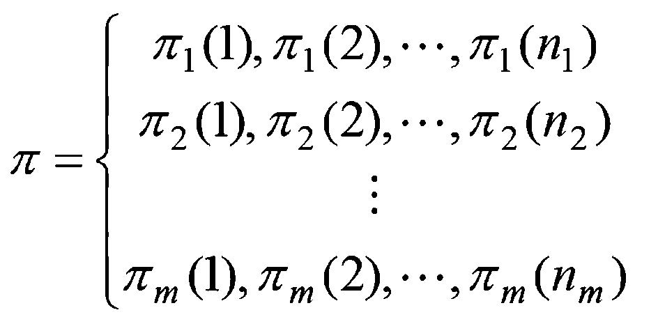
A. Solution RepresentationThe population is composed by a set of solutions for the UPMSP-SDST. A solution is represented by $m$ job sequences as illustrated in Fig. 1. Each sequence represents the order of processing jobs on the corresponding machine. For example,element $\pi_{k}(i)$ implies that $J_{\pi_{k}(i)}$ is the $i$-th job on $M_{k}$.

|
Download:
|
| Fig. 1 Solution representation in the EDA-IG. | |
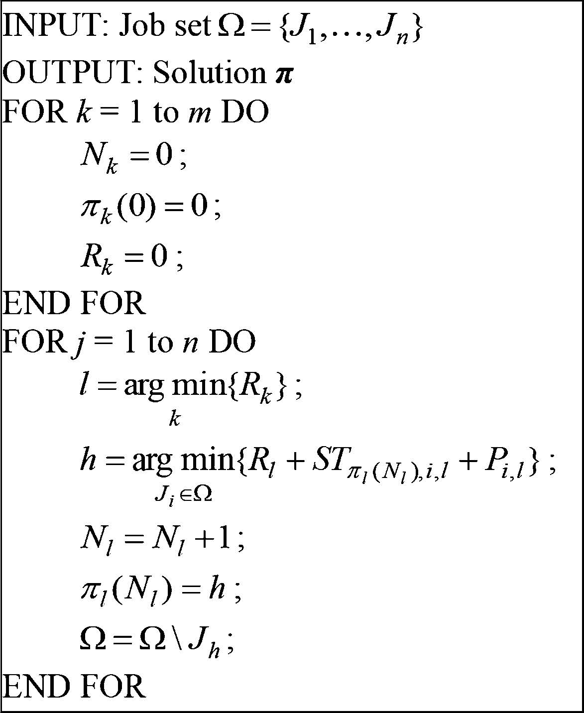
Considering both the quality and diversity of initial solutions, the smallest release-time and earliest completion (SR EC) rule is employed for initialization. To be specific,to determine the job sequences on the machines,it selects a machine with the smallest release-time and assigns an unprocessed job which results in the earliest completion time of the machine. If more than one machine or job meets the requirement,it randomly selects one from them. A new solution is obtained after all the jobs are assigned. The pseudo code to generate an initial solution is shown in Fig. 2.

|
Download:
|
| Fig. 2 The procedure to generate an initial solution. | |
With the above procedure, a total of $Psize$ initial solutions are generated. Because the SR EC rule is a greedy assignment, it is helpful to obtain a solution with a small makespan. Meanwhile, when generating a new solution, initial release times of all the machines are the same, i.e., zero. Hence, the order of the first $m$ assigned machines is random, which ensures the diversity of initial solutions. Therefore, the initialization mechanism is beneficial to both the quality and diversity of initial solutions.
C. Probability Model and Updating MechanismThe crucial factor of the EDA is the probability model that describes the distribution of the search space. Usually, the probability model is built according to the characteristics of the elite solutions. For the UPMSP-SDST, the neighboring relations of the jobs on the machines affect the makespan of the solution. Therefore, a probability model is designed as $m$ probability matrices as follows:
| \begin{equation} P^{k}(g)= \left[ \begin{matrix} p_{01}^{k}(g) & p_{02}^{k}(g) & \dots & p_{0n}^{k}(g)\\ 0 & p_{12}^{k}(g) & \dots & p_{1n}^{k}(g)\\ p_{21}^{k}(g) & 0 & \dots & p_{2n}^{k}(g)\\ \vdots & \vdots & \ddots & \vdots\\ p_{n1}^{k}(g) & p_{n2}^{k}(g) & \dots & 0 \end{matrix} \right] ,k=1,2,\dots,m, \end{equation} |
where $p_{ij}^{k}(g)$ represents the probability that $J_{j}$ is right after $J_{i}$ on $M_{k}$ at the $g$-th generation. Besides, $p_{0j}^{k}(g)$ represents the probability that $J_{j}$ is the first job on $M_{k}$ . Note that,$\forall j,g,p_{jj}^{k}(g)=0$.
The matrices are initialized uniformly as follows:
| \begin{equation} P^{k}(0)= \left[ \begin{matrix} 1/n & 1/n & \dots & 1/n\\ 0 & 1/(n-1) & \dots & 1/(n-1)\\ 1/(n-1) & 0 & \dots & 1/(n-1)\\ \vdots & \vdots & \ddots & \vdots\\ 1/(n-1) & 1/(n-1) & \dots & 0 \end{matrix} \right] ,\forall k. \end{equation} | (10) |
At each generation, the probability matrices are updated by the information of some elite solutions of the population. The elite sub-population consists of the best $SPsize$ solutions, where $SPsize=\eta\,\%Psize$. To be specific, the updating process can be regarded as the following incremental learning:
| \begin{equation} p_{ij}^{k}(g+1)=(1-\alpha)p_{ij}^{k}(g)+\frac{\alpha}{SPsize}\sum\limits_{s=1}^{SPsize}I_{ijk}^{s}(g), \end{equation} | (11) |
where $\alpha \in(0,1)$ is the learning rate,and $I_{ijk}^{s}(g)$ is the indicator function corresponding to the $s$-th solutions of the elite sub-population.
| \begin{equation} I_{ijk}^{s}(g)= \begin{cases} 1,& \text{if $J_{j}$ is right after $J_{i}$ on $M_{k}$},\\ 0,& \text{else}. \end{cases} \end{equation} | (12) |
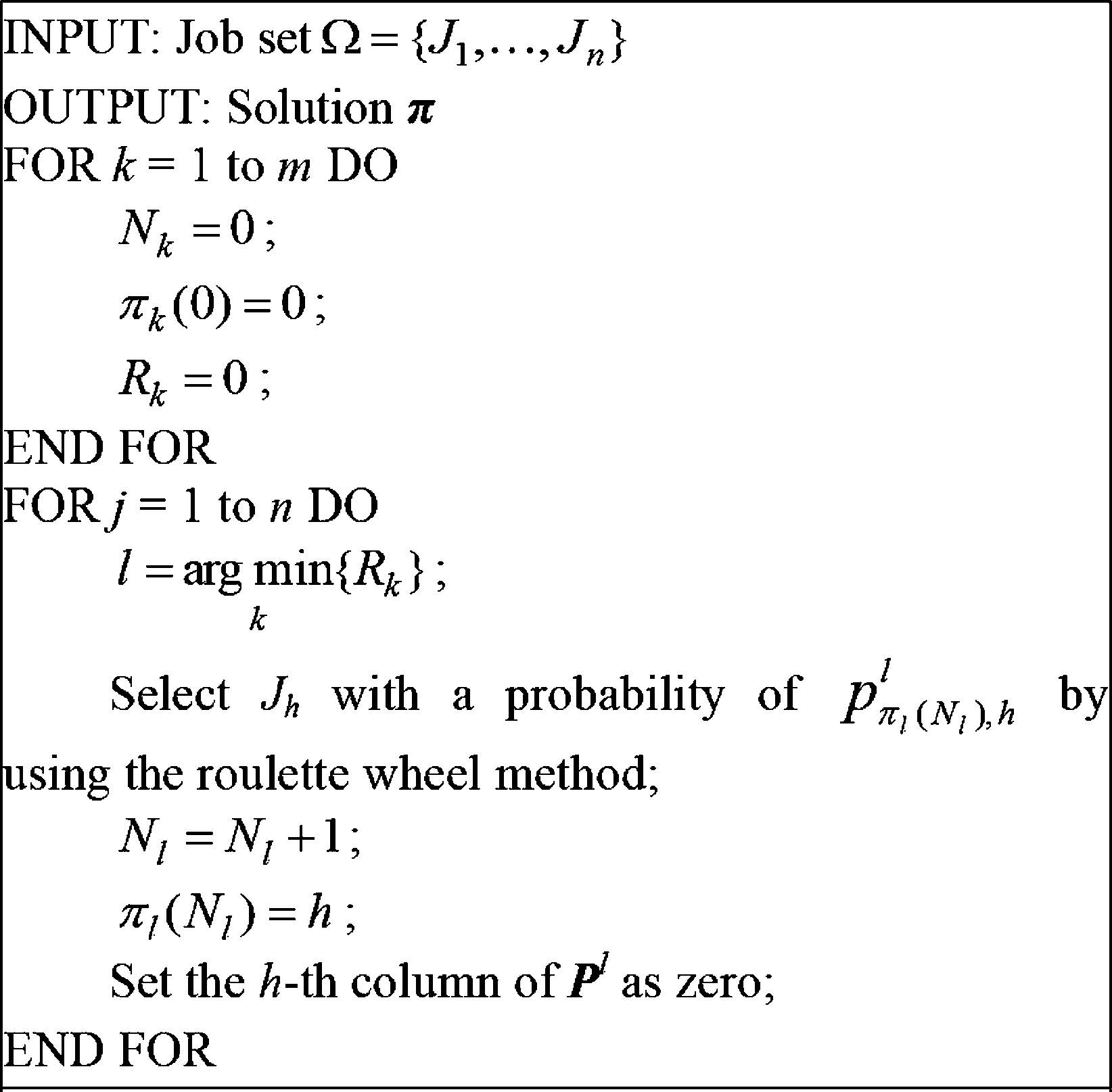
Then, new solutions are generated by sampling the probability matrices. To generate a solution, the jobs are assigned to machines one by one. For a machine with the smallest release-time, a job is selected by using the roulette wheel method. The procedure to generate a solution by sampling the probability model is illustrated in Fig. 3.

|
Download:
|
| Fig. 3 The procedure to generate a solution by sampling. | |
The EDA pays much attention to global exploration while its exploitation capability is relatively limited. Therefore, an IG search is developed to enhance the local exploitation of the EDA.
The IG method was introduced by Ruiz and St${\rm \ddot{u}}$tzle[26] and has been applied for the UPMSP without SDST[7]. The IG method starts from a schedule and iterates three phases: deconstruction, reconstruction, and improvement. First, some jobs are randomly removed in the deconstruction phase. Then, these jobs are reassigned one by one in a greedy way in the reconstruction phase. Afterwards, local search operators are implemented in the improvement phase. If the new solution is better, it will replace the old one; else, the next iteration starts from the old solution.
For the UPMSP-SDST, two types of IG method (named IG1 and IG2 respectively) are developed. The three phases of IG1 and IG2 are introduced as follows:
1) Deconstruction phase.
IG1: For each machine, randomly select a job and remove it.
IG2: For each machine, randomly select a job and remove all the jobs after it.
2) Reconstruction phase.
IG1: Suppose to insert each removed job into every position on all the machines. Record the job and the position which result in the smallest makespan. Then, insert the job into the position. Repeat the procedure until all the removed jobs are reassigned.
IG2: Reassign all the removed jobs based on the SR EC rule.
3) Improvement phase.
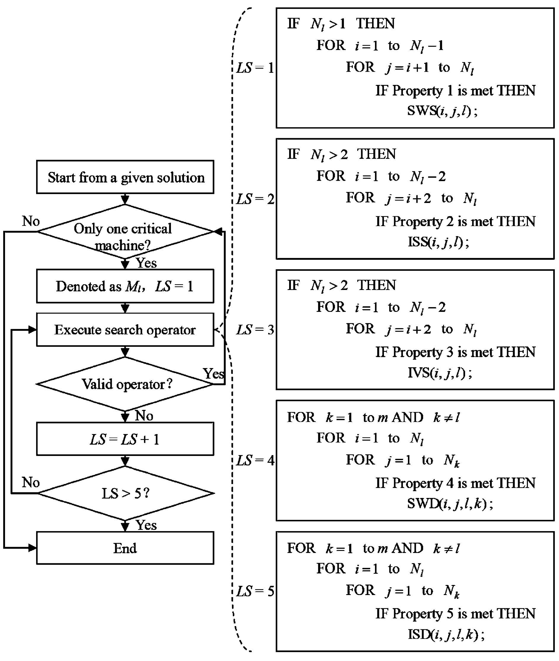
The improvement phases of IG1 and IG2 are the same. If the solution obtained in the reconstruction phase has only one critical machine, neighborhood search operators are executed one after another. Besides, Properties 1-5 are used to avoid invalid operators. The procedure of the improvement phase is illustrated in Fig. 4.

|
Download:
|
| Fig. 4 The procedure of the improvement phase. | |
At each generation of the EDA-IG, IG search is implemented on the best solution of the population. Considering search sufficiency and computation budget, IG search iterates until the solution has not been updated in $\gamma$ continuous iterations. Parameter $\gamma$ implies the intensity of the local exploitation. The parameter setting for $\gamma$ will be investigated later,and a rule for selecting a type of IG according to the job and machine numbers will be presented as well.
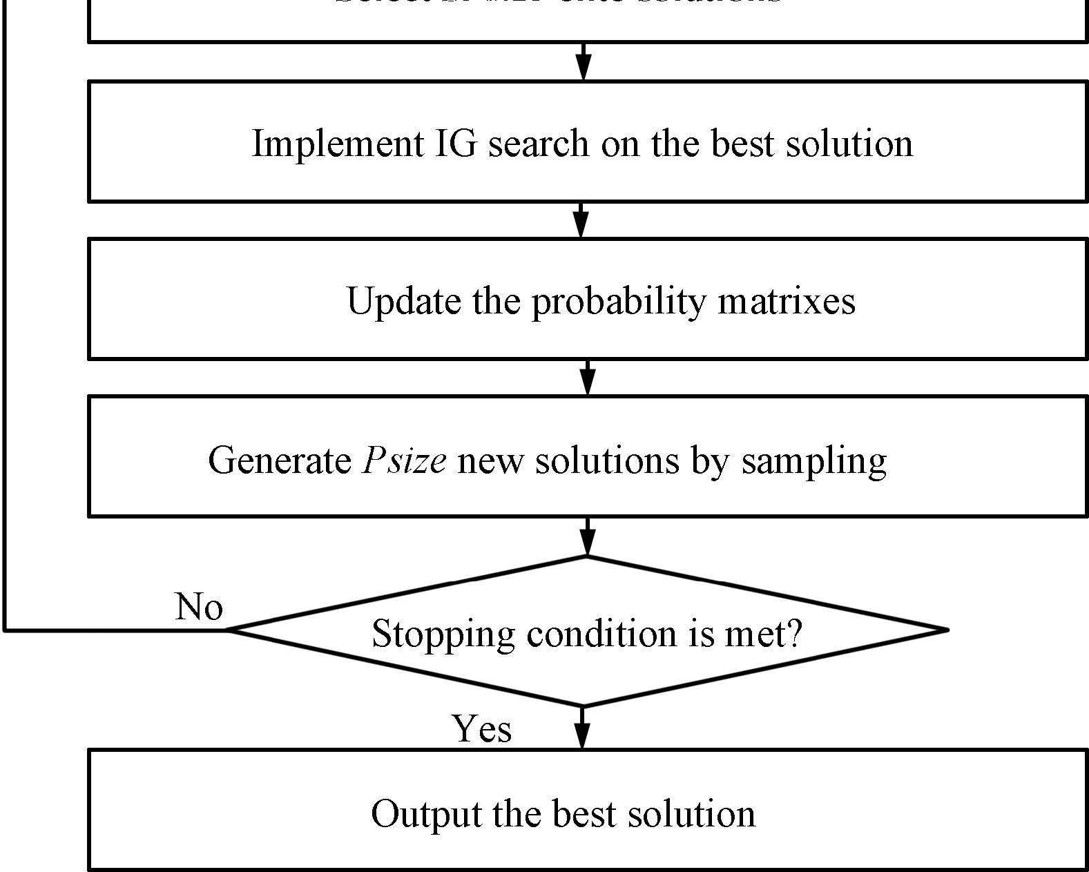
E. Flowchart of EDA-IGWith the above design, the flowchart of the EDA-IG for solving the UPMSP-SDST is illustrated in Fig. 5.

|
Download:
|
| Fig. 5 The flowchart of the EDA-IG. | |
At the initial stage of evolution process, the whole search space is sampled uniformly. Then, the algorithm uses the EDA-based evolutionary search mechanism to sample a potential area. Moreover, IG search is implemented in a promising region, aiming to obtain better solutions. With the benefit of combining EDA and IG search, global exploration and local exploitation are balanced. The stopping criterion is set with a maximum elapsed CPU time of $n\times(m/2) \times t$ ms.
F. Computational Complexity AnalysisFor each generation of the EDA-IG, the computational complexity can be roughly analyzed as follows:
1) EDA: For the updating process, first it is with a computational complexity of O($Psize \cdot$ log$Psize$) by using the quick sorting method to sort and select elite solutions; then, it is with a computational complexity of O$[n\cdot (Psize+m\cdot n)]$ to update the probability matrices. For the sampling process, it generates a new solution with a computational complexity of O$[n\cdot(m+n)]$.
2) IG: The deconstruction phase is with a computational complexity of O$(m)$. The reconstruction phases of IG1 and IG2 are with computational complexities of O$(m^{2}\cdot n)$ and O$[n\cdot (m+n)]$,respectively. The improvement phase is with a computational complexity of O$(n^{2})$. Therefore, the computational complexities of IG1 and IG2 are O$(m^{2}\cdot n+n^{2})$ and O$(m\cdot n+n^{2})$,respectively. Note that,IG2 needs less computation budget than IG1.
Ⅴ. NUMERICAL RESULTS AND COMPARISONSTo test the performance of the EDA-IG, numerical tests are carried out with two sets of benchmark instances[10], which are available at http://soa.iti.es. The first set consists of 640 small-scale instances, where $n$ = {6,8,10,12} and $m $= {2, 3,4,5}. The second set consists of 1000 large-scale instances, where $n$ = {50,100,150,200,250} and $m$ = {10,15,20,25, 30}. The processing times are uniformly distributed between 1 and 99. The setup times consist of four sub-sets, which are uniformly distributed between 1-9, 1-49, 1-99 and 1-124, respectively.
To evaluate the performance of the EDA-IG, same as the literature[10], the experimental results are evaluated by relative percentage deviation (RPD) as follows:
| \begin{equation} \text {RPD}=\frac{alg-opt}{opt}\times 100. \end{equation} | (13) |
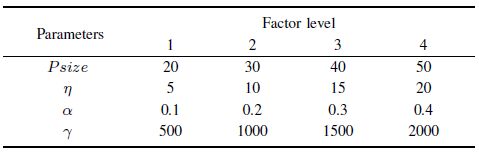
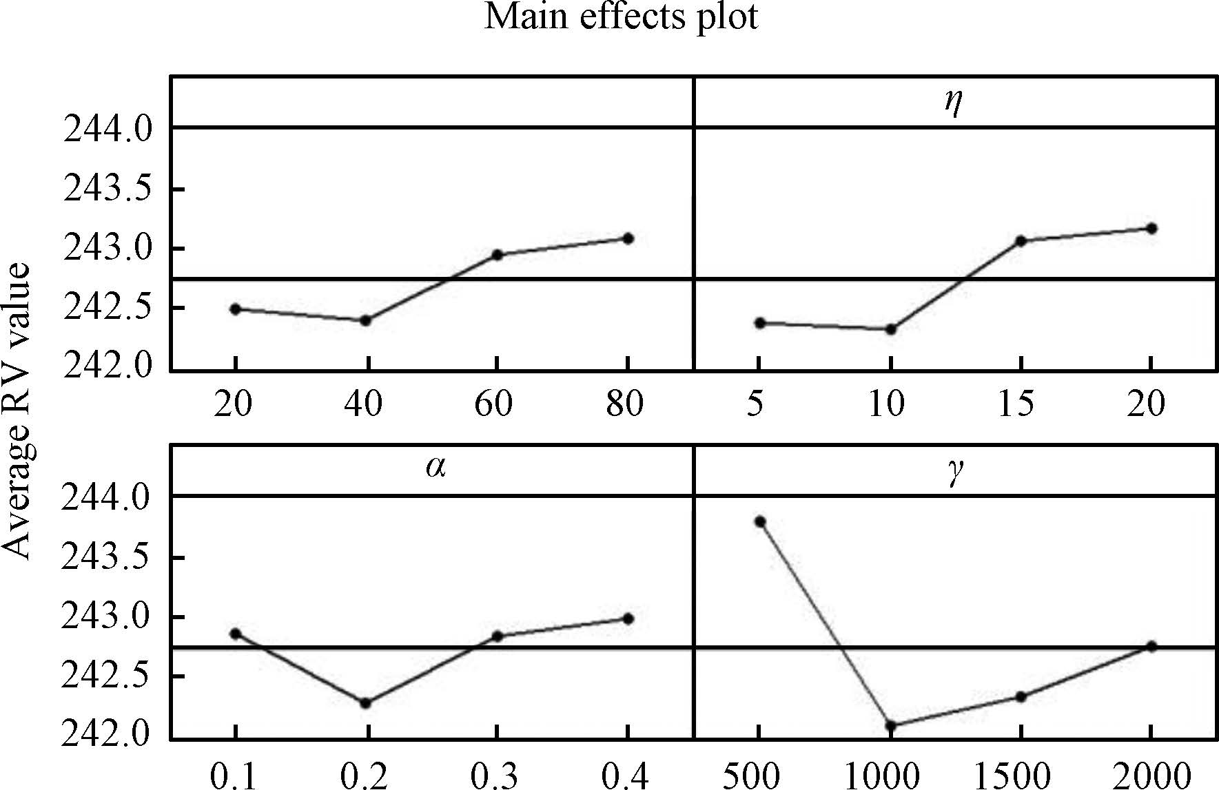
The EDA-IG has four key parameters to be set: $Psize$ (population size),$\eta$ (percentage of elite solutions),$\alpha$ (learning rate),and $\gamma$ (intensity of IG search). To investigate the influence of these parameters on the performance of the EDA-IG, the Taguchi method of design-of-experiment (DOE)[28] is implemented by using a moderate-scale instance I_100_10_S_1-124_1. Besides, the stopping criterion is set with a maximum elapsed CPU time of $n\times(m/2)\times30$ ms, and IG2 method is used in the EDA-IG.
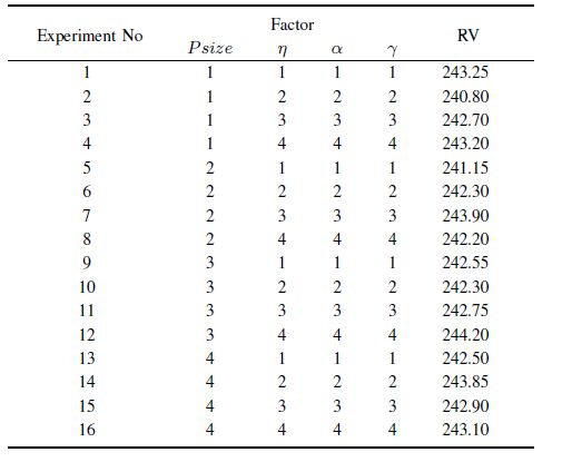
Four factor levels are employed. Different values of these parameters are listed in Table I. Accordingly, the orthogonal array $L_{16}(4^{4})$ is chosen. For each parameter combination, the EDA-IG is run 20 times independently and the average RPD value of 20 runs is obtained as the response variable (RV) value. The orthogonal array and RV values are listed in Table II.
|
|
Table Ⅰ FACTOR LEVEL OF PARAMETERS |
|
|
Table Ⅱ THE RV VALUE |
According to the orthogonal table,the influence trend of each parameter is illustrated in Fig. 6. The average RV values of each parameter are figured out to analyze the significance rank. The results are listed in Table Ⅲ.

|
Download:
|
| Fig. 6 The influence trend of each parameter. | |
|
|
Table Ⅲ RESPONSE TABLE |
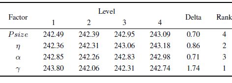
From Fig. 6 and Table III,it can be seen that all the parameter values should be neither too small nor too large. Besides,the intensity of IG search has the most significant impact. A small value of $\gamma$ could not provide sufficient local exploitation while a large value may waste the computation budget. The significance of $\eta$ ranks the second. A proper value is helpful to update the probability model efficiently. The significance of $\alpha$ ranks the third. A small value of $\alpha$ could lead to slow convergence while a large value could lead to premature convergence. Although $Psize$ has the slightest influence,a small value cannot provide enough search breadth while a large value may cause insufficient evolution due to fewer generations. According to the analysis,the suggested values are as follows: $Psize = 40, \eta = 10,\alpha = 0.2,\gamma = 1000$. This setting is also used in the following experiments.
B. Effectiveness of Hybrid StrategyTo show the effectiveness of hybridizing EDA and IG search, the performances of EDA, IG1, IG2, EDA-IG1, and EDA-IG2 are compared by using the first set of benchmark instances. EDA has no IG search while the IG1 and IG2 have no EDA-based search, i.e., the learning rate is zero. EDA-IG1 and EDA-IG2 denote the EDA with IG1 and IG2, respectively. For fair comparison, the parameter values are the same and the stopping criterion is set with a maximum elapsed CPU time of $n\times(m/2) \times10$ ms for all the algorithms. The algorithms are run 5 times independently and the smallest RPD values are obtained. Table IV summarizes the results grouped by $n$ (160 data per average).
|
|
Table Ⅳ COMPARISON OF EDA, IG1, IG2, EDA-IG1 AND EDA-IG2 |
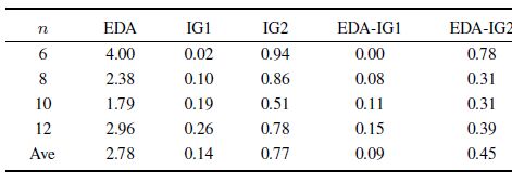
From Table IV, it can be seen that EDA-IG1 outperforms EDA and IG1 while EDA-IG2 outperforms EDA and IG2. Therefore, it can be concluded that EDA-IG is better than both EDA and IG, which shows that the hybrid strategy is effective. Besides, EDA-IG1 is the best one of the five algorithms for the small-scale instances.
C. Selection Rule of IG MethodsTo further investigate the effect of different IG methods, performances of EDA-IG1 and EDA-IG2 are compared based on the second set of benchmark instances. The stopping criterion is set with a maximum elapsed CPU time of $n\times(m/2) \times30$ ms. The two algorithms are run 5 times independently and the smallest RPD values are obtained. Table V summarizes the results grouped by each combination of $n$ and $m$ (40 data per average).
|
|
Table Ⅴ COMPARISON OF EDA, IG1, IG2, EDA-IG1 AND EDA-IG2 FOR LARGE-SCALED INSTANCES |
From Table V,it can be seen that EDA-IG1 outperforms EDA-IG2 when $n\times m$ is small, and EDA-IG2 outperforms EDA-IG1 when $n\times m$ is large. The reasons are as follows: In the reconstruction phase, IG1 searches every possible position for each removed job while IG2 assigns a job to the last position of a machine. Hence, IG1 explores more search space than IG2. Accordingly, the local exploitation ability of EDA-IG1 is stronger than that of EDA-IG2. Meanwhile, the computational complexity of IG1 is larger than that of IG2. When the scale of instance is larger, EDA-IG2 can evolve much more generations than EDA-IG1. Therefore, EDA-IG1 is better for small-scale instances and EDA-IG2 is better for large-scale ones.
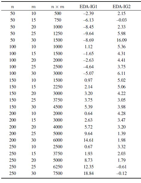
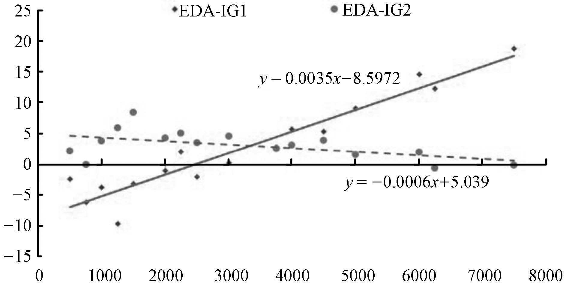
To investigate the selection rule of IG methods, the average result for each combination of $n\times m$ is illustrated in Fig. 7. For example, when $n\times m = 1500$,the value is an average result of $\{n = 50,m = 30\}$,$\{n = 100,m = 15\}$,and $\{n = 150,m = 10\}$.

|
Download:
|
| Fig. 7 Comparison of EDA-IG1 and EDA-IG2 for different values of n × m. | |
The linear least square method is utilized to determine the relationship between average RPD ($y$-axis) and the value of $n\times m$ ($x$-axis). The tropic equations for EDA-IG1 and EDA-IG2 are $y=0.0035x-8.5972$ and $y=-0.0006x+5.039$,respectively. The abscissa of the intersection point is about 3325.9. Therefore,the selection rule of IG methods is as follows: If $n\times m<3326$, IG1 is employed in EDA-IG; else, IG2 is employed. Such a selection rule will be used in the following numerical tests.
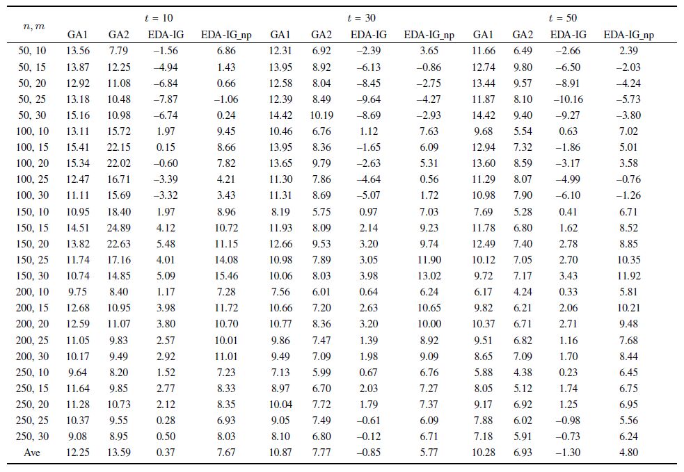
D. Comparison with Existing Algorithms and EDA-IG Without the PropertiesNext, the EDA-IG is compared with two GAs[10]. Moreover, to verify the effectiveness of proposed five properties by numerical experiments, the EDA-IG is compared with the EDA-IG without using the properties (denoted as EDA-IG_np). For the 640 small-scaled and 1000 large-scale benchmark instances, Vallada and Ruiz provided best-known solutions accordingly[10]. Same as [10], EDA-IG and EDA-IG_np are run 5 times independently for each instance. Besides, the best RPD values are obtained for three $t$ values, which represent the performances of different CPU times. Tables Ⅵ and Ⅶ summarize the results grouped by each combination of $n$ and $m$ (40 data per average) as in [13],where the results of the GAs are directly from the literature.
|
|
Table Ⅵ COMPARISON AMONG GAs, EDA-IG, AND EDA-IG NP FOR SMALL-SCALED INSTANCES |
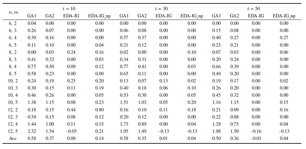
From Tables Ⅵ and Ⅶ, it can be seen that EDA-IG outperforms EDA-IG_np for solving both the small- and large-scale instances. As the problem scale increases, the superiority of EDA-IG becomes more obvious. For the small-scale instances, the average result of EDA-IG is better than that of EDA-IG_np for each CPU time. For the large-scale instances, the average result of EDA-IG_np within a relatively large amount of CPU time ($t$ = 50) is even worse than that of EDA-IG within a relatively short amount of CPU time ($t$ = 10). Thus, the results demonstrate that the proposed properties can truly save the computational time to a great extent.
|
|
Table Ⅶ COMPARISON AMONG GAs, EDA-IG, AND EDA-IG NP FOR LARGE-SCALED INSTANCES |
Compared with the GAs, EDA-IG performs better for solving both the small- and large-scale instances. For the small-scale instances, the average result of EDA-IG is 0.09 within a relatively short amount of CPU time ($t$ = 10). After a relatively large amount of CPU time ($t$ = 50), the average result of EDA-IG is $-$0.01 while the one of GA1 is 0.50 and the one of GA2 is 0.36. Within such amount of CPU time, EDA-IG updates the best-known solution of one small-scale instance. For the large-scale instances, the superiority of EDA is more obvious. The average result of EDA-IG is 0.37 within a relatively short amount of CPU time ($t$ = 10). After a relatively large amount of CPU time ($t$ = 50), the average result of EDA-IG is $-$1.30 while the one of GA1 is 10.28 and the one of GA2 is 6.93. Within such amount of CPU time, EDA-IG updates the best-known solutions of 530 large-scaled instances.
With above numerical tests, it can be concluded that the proposed EDA-IG and the derived properties are effective for solving the UPMSP-SDST.
VI. CONCLUSIONIn this paper, an EDA-IG is proposed to solve the UPMSP-SDST with the objective of minimizing the makespan. The contributions of this work can be summarized as follows:
1) Some properties for judging the effectiveness of neighborhood search operators are derived. These properties can be used to avoid invalid search and to speed up the evaluation of new solutions in the EDA-IG. Besides, these properties can be employed to develop effective strategies for local search in designing other algorithms.
2) Based on the neighbor relations of the jobs, a probability model is built to describe the distribution of the search space. It helps the algorithm to generate new solutions by sampling a promising search region.
3) To enhance the exploitation, a special IG search is developed to improve the best solution of the population. Two types of deconstruction and reconstruction are designed, and a selection rule is presented.
4) Numerical tests and comparisons with 1640 benchmark instances show that the EDA-IG outperforms the existing GAs. Meanwhile, the best-known solutions of 531 instances are updated by the EDA-IG. Besides,the effectiveness of the derived properties is also verified by comparisons.
Future work could focus on developing the learning-based EDA-IG algorithm by adaptively using multiple search operators. It is also interesting to study the specific EDA-IG algorithm for the distributed scheduling problems by investigating the problem-specific information.
| [1] | Cheng T C E, Sin C C S. A state-of-the-art review of parallel-machine scheduling research. European Journal of Operational Research, 1990, 47(3): 271-292 |
| [2] | Chen J, Pan Q K, Wang L, Li J Q. A hybrid dynamic harmony search algorithm for identical parallel machines scheduling. Engineering Optimization, 2012, 44(2): 209-224 |
| [3] | Xu Y, Wang L, Wang S Y, Liu M. An effective shuffled frog-leaping algorithm for solving the hybrid flow-shop scheduling problem with identical parallel machines. Engineering Optimization, 2013, 45(12): 1409-1430 |
| [4] | Lin S W, Ying K C. A multi-point simulated annealing heuristic for solving multiple objective unrelated parallel machine scheduling problems. International Journal of Production Research, 2015, 53(4): 1065-1076 |
| [5] | Mellouli R, Sadfi C, Chu C B, Kacem I. Identical parallel-machine scheduling under availability constraints to minimize the sum of completion times. European Journal of Operational Research, 2009, 197(3): 1150-1165 |
| [6] | Xu X Q, Lin J, Cui W T. Hedge against total flow time uncertainty of the uniform parallel machine scheduling problem with interval data. International Journal of Production Research, 2014, 52(19): 5611-5625 |
| [7] | Fanjul-Peyro L, Ruiz R. Iterated greedy local search methods for unrelated parallel machine scheduling. European Journal of Operational Research, 2010, 207(1): 55-69 |
| [8] | Garey M R, Johnson D S. Computers and Intractability: A Guide to the Theory of NP-completeness. San Francisco, USA.: W.H. Freeman & Co., 1979. |
| [9] | Allahverdi A, Ng C T, Cheng T C E, Kovalyov M Y. A survey of scheduling problems with setup times or costs. European Journal of Operational Research, 2008, 187(3): 985-1032 |
| [10] | Vallada E, Ruiz R. A genetic algorithm for the unrelated parallel machine scheduling problem with sequence dependent setup times. European Journal of Operational Research, 2011, 211(3): 612-622 |
| [11] | Behnamian J, Zandieh M, Fatemi Ghomi S M T. Parallel-machine scheduling problems with sequence-dependent setup times using an ACO, SA and VNS hybrid algorithm. Expert Systems with Applications, 2009, 36(6): 9637-9644 |
| [12] | Chang P C, Chen S H. Integrating dominance properties with genetic algorithms for parallel machine scheduling problems with setup times. Applied Soft Computing, 2011, 11(1): 1263-1274 |
| [13] | Fleszar K, Charalambous C, Hindi K S. A variable neighborhood descent heuristic for the problem of makespan minimisation on unrelated parallel machines with setup times. Journal of Intelligent Manufacturing, 2012, 23(5): 1949-1958 |
| [14] | Lin S W, Ying K C. ABC-based manufacturing scheduling for unrelated parallel machines with machine-dependent and job sequence-dependent setup times. Computers & Operations Research, 2014, 51: 172-181 |
| [15] | Yilmaz E D, Ozmutlu H C, Ozmutlu S. Genetic algorithm with local search for the unrelated parallel machine scheduling problem with sequence-dependent set-up times. International Journal of Production Research, 2014, 52(19): 5841-5856 |
| [16] | Arnaout J P, Rabadi G, Musa R. A two-stage ant colony optimization algorithm to minimize the makespan on unrelated parallel machines with sequence-dependent setup times. Journal of Intelligent Manufacturing, 2010, 21(6): 693-701 |
| [17] | Avalos-Rosales O, Angel-Bello F, Alvarez A. Efficient metaheuristic algorithm and re-formulations for the unrelated parallel machine scheduling problem with sequence and machine-dependent setup times. The International Journal of Advanced Manufacturing Technology, 2015, 76(9-12): 1705-1718 |
| [18] | Chen J F. Scheduling on unrelated parallel machines with sequenceand machine-dependent setup times and due-date constraints. The International Journal of Advanced Manufacturing Technology, 2009, 44(11-12): 1204-1212 |
| [19] | Lin S W, Lu C C, Ying K C. Minimization of total tardiness on unrelated parallel machines with sequence-and machine-dependent setup times under due date constraints. The International Journal of Advanced Manufacturing Technology, 2011, 53(1-4): 353-361 |
| [20] | Hsu C J, Kuo W H, Yang D L. Unrelated parallel machine scheduling with past-sequence-dependent setup time and learning effects. Applied Mathematical Modelling, 2011, 35(3): 1492-1496 |
| [21] | Kuo W H, Hsu C J, Yang D L. Some unrelated parallel machine scheduling problems with past-sequence-dependent setup time and learning effects. Computers & Industrial Engineering, 2011, 61(1): 179-183 |
| [22] | Joo C M, Kim B S. Hybrid genetic algorithms with dispatching rules for unrelated parallel machine scheduling with setup time and production availability. Computers & Industrial Engineering, 2015, 85: 102-109 |
| [23] | Chen C L, Chen C L. Hybrid metaheuristics for unrelated parallel machine scheduling with sequence-dependent setup times. The International Journal of Advanced Manufacturing Technology, 2009, 43(1-2): 161-169 |
| [24] | Larrañaga P, Lozano J A. Estimation of Distribution Algorithms: A New Tool for Evolutionary Computation. US: Springer, 2002. |
| [25] | Ceberio J, Irurozki E, Mendiburu A, Lozano J A. A review on estimation of distribution algorithms in permutation-based combinatorial optimization problems. Progress in Artificial Intelligence, 2012, 1(1): 103-117 |
| [26] | Ruiz R, StÄutzle T. A simple and effective iterated greedy algorithm for the permutation flowshop scheduling problem. European Journal of Operational Research, 2007, 177(3): 2033-2049 |
| [27] | Guinet A. Scheduling sequence-dependent jobs on identical parallel machines to minimize completion time criteria. International Journal of Production Research, 1993, 31(7): 1579-1594 |
| [28] | Montgomery D C. Design and Analysis of Experiments (Seventh Edition) . New York, U. S. A.: John Wiley & Sons, 2008. |