Ⅰ. INTRODUCTION

Wireless sensor network (WSN) is currently a hot research field,and has broad applications in target tracking^[1],surveillance^[2] and environment monitoring^[3],etc. Due to its extraordinarily limited resource,storage capacity and processing power,single sensor may easily lead to poor stability,slow convergence and low monitoring accuracy. By contrast,multiple sensors can cover more areas and provide views from different angles,and the fusion of all measurements may lead to a more complete scene understanding. To solve inadequacy of a single sensor,information fusion technology has become an effective means. Usually,there are two basic structure for the information systems,which are composed by centralized and distributed fusion approaches. The centralized approaches may be unreliable and have less accuracy and stability when a severe fused data fault occurs. While,distributed fusion algorithms have various advantages,e.g.,relatively lower demand for resources,higher fault tolerance,better network scalability, better real-time performance and stronger stability,which always raises great concern^{[4, 5]}.

Kalman filter algorithm is a classic method for state estimation in WSN,and researches on consistency lay the foundations for distributed computing^[6]. Great efforts are made to design distributed estimation algorithms,which combine a consensus filter and a Kalman filter. The methods ensure that the estimates asymptotically converge to the same value. Consensus based estimation does not rely on one single sensor,but each sensor estimates the state of dynamical system,and exchanges the estimates and measurements among neighbors. Such algorithms emerge as effective tools for solving a wide variety of data fusion problems in sensor network. A typical example of such algorithm was proposed in [7],by applying consensus filter to fuse sensor measurements and covariance for improving node estimation performance. The algorithm had a satisfactory stability,however,there also existed distinct distributed estimation problems. For example,too much information transmission may lead to slow convergence of the algorithm and weak anti-disturbance ability when network size is increasing. Further extension of the work in [7] can be found in [8, 9]. A consensus-based distributed filtering algorithm was also presented in [10],which was guaranteed to be globally asymptotically stable. All of these algorithms could effectively achieve optimal estimation of other unknown parameters. However,all algorithms assumed that each node configured an equal certainty degree without taking into account the differences between nodes. In reality,there may be certain observation differences,inevitably environmental interferences,and unknown node position in sensor network topology, etc. Therefore,how to assign reasonable weights for multiple sensors becomes a key problem for multi-information fusion. For solving such a problem,in [11],the authors introduced a method to optimize consensus weights by fusing estimates from the neighbors to enhance the consistency of the state estimates,in while each step taken a long time to adjust the weights. In [12],making use of node degree on estimation performance,the authors proposed a quantization function to optimize the consensus protocol.~ Specially,in [13],it should be noted that giving higher weights to the nodes with better information of the network was reasonable. In [14],a spatially distributed variable tap-length algorithm was presented to track and estimate unknown parameter vectors and weights. The algorithm in [15] introduced a criterion to optimize the weights in consensus algorithm and proved that mean squared deviation of node states was a convex function of the weights. A basic assumption in this research is that sensor data is reliable. However,in the literature,few results are explicitly considered. Since sensor nodes are exposed to non-controlled circumstances and vulnerable to be attacked,which may easily lead to information tampered and falsified in process of the information transfer,and may ultimately affect estimation performance of the target positioning and tracking.

Our main object is to propose a distributed filtering algorithm based on tunable weights under untrustworthy dynamics. Firstly,an evaluation algorithm is introduced to calculate the certainty degree of the neighbors based on the node location in network topology,and then quantitative value is used to optimize consensus protocol as a fusion weight to update node status estimates. Secondly,on the basis of load redistribution in complex network theory of ^{[16, 17]},the attacked node weights are redistributed to the neighbors to enhance their estimation accuracy. Simulations are conducted under the random attack model and selective attack model to verify and demonstrate our methods.

Ⅱ. PROBLEM STATEMENT

We are interested in tracking state of target using a sensor network with communication topology $G=(V,E)$. The graph $G$ consists of a set of vertices $V=\{1,2,\ldots,n\}$ and a set of edges $E=\{e_{ij}\}$. The graph $G$ is undirected and each vertex corresponds to a sensor. The set of neighbors $N_i$ of sensor $V_i$ is given by $N_i=\{V_j:(V_i,V_j)\in E\}$. Consider WSN with $n$ sensors deployed to track a real $m\times1$ random vector $x(t)$ $ \in {{\rm{R}}^{m \times 1}}$. The dynamic process is represented by the following linear time-varying model:

$ \begin{align} x(t+1)=Ax(t)+\omega(t), \end{align} $

(1)

where $A\in {\bf R}^{m\times m}$,and driving input $w(t)\in {\bf R}^{m\times1}$ is a zero-mean white Gaussian noise with covariance matrix $Q>0$,and $E( w(k) w(l)^{\rm T})$ $=$ $Q(k)\delta (k - l)$^[18]. We model observation $z(t)$ $\in$ ${\bf R}^{m\times1}$ at time $t$ as

$ \begin{align} z_i(t)=H_ix(t)+v_i(t), \end{align} $

(2)

where $H_i\in {\bf R}^{m\times m}$ and observation noise $v_i(t)\in {\bf R}^{m\times1}$ is a zero-mean Gaussian with covariance matrix $R>0$,and $E( v_i(k),v_j(l)^{\rm T})= R_i(k)\delta(i-j)\delta(k-l) $. $\delta(t) $ is Dirac delta function,where $\delta(\tau)=1 $ if $\tau=0 $,and $\delta(\tau)=0 $,otherwise.

We are interested in the problem of distributed estimation of the state $x$ in (1),in which a number of nodes generate their estimates based on the measurements in (2). When performing in an untrustworthy environment,some sensors may experience failure, and thus have no access to the measurement of the target or have tampered and falsified information of the target. Each node is only allowed to communicate with its neighbors and only once between each measurement,the sensors are modeled by

$ \begin{align} z_i=\mu H_ix+v_i, \end{align} $

(3)

where attack coefficient $\mu$ reflects different degree of network on a regular basis. Contrast to a correct observation model (2),it can be seen that $\mu=1$ means no attacks,the coefficient $\mu$ departs from 1 further and it effects deeply.

In this paper,a general case is considered that each node has different estimation ability,and sensor node transmits and receives the data expected to be reliable.

In summary,the contributions of our paper are:

1) Designing an algorithm to evaluate node estimation ability;

2) Reducing the influence of the abnormal data on the final result of the data fusion and getting a good estimate $\hat x_i$ of the state $ x$ under untrustworthy dynamics.

Ⅲ. DISTRIBUTED ALGORITHM BASED ON TUNABLE WEIGHTS A. Consensus Protocol

Consensus protocol defines a rule that each node tends to global consistent state due to the interaction. Xiao designed a class of an average consensus iterative algorithm in [19],and analyzed convergence by semi-definite convex programming method. The iterative equation is:

$ \begin{align} x_i(t+1)=W x_i(t). \end{align} $

(4)

Two different weighted methods hold:

1) Fixed-edge weighted method. $W$ can be calculated by the following $W=I-a L$,where $a$ is a positive constant;

2) Metropolis weighted method. Edge weights are based on maximum-degree of the neighbors. Equation $W_{ij}=(1+\max \{d_i, d_j\})^{-1}$ is calculated,followed by choosing $W_{ii}$,$W1$ $=$ $\bf 1$.

Based on weighted equation (4),the system eventually converges to: $\lim\nolimits_{t \to \infty }{x_i(t+1)}=\lim\nolimits_{t \to \infty }W^t{x(0)}=((1/n){\bf 11}^{\rm T})x(0)$. Here ${\bf 1}$ denotes the vector with all coefficients being one.

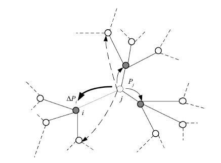
B. Weights Redistribution

In the filtering problem,it is assumed that each sensor node has an equal certainty degree of locating a target. However,each node at different location with different neighbors may cause different influences on the WSN. As we all know,due to external disturbance and inevitable model error in real applications,each node has different certainty degree of locating a target ultimately. When a sensor node is attacked,the higher weight the node has,the larger the influence over the sensor network is,so to some extent,failure nodes may impact the estimation performance of the sensor network. Consider the load redistribution in real-world complex networks,when traffic accidents occur in road intersection of urban transport networks,some vehicles may have to re-plan and make another choice. As to the transport network, vehicles may prefer intersections which are closer to the failed nodes when reconfiguring the route. It means removing one node or one edge may lead its load to redistribute to its neighbors in the region complex network. Our main objective is to draw on this idea. We regard the load as a node certainty degree of locating a target. In quest of ensuring the estimation accuracy of the WSN, the attacked node weights are redistributed to improve other intact node certainty degree,which ultimately minimizes the sensor network losses.

To begin with,we propose the equation of node certainty degree, and then give each node different certainty degree of locating a target. Afterwards,the main computing processes of the proposed algorithm are given.

Definition 1. The distance $\ell_{ij}$ between $V_i$ and $V_j$ is defined as the weight of edge $e_{ij}$. Assume a set of sensors $[V_k,V_i]$ and a set of edges constitute an alternating sequence $\Delta=V_ie_{ij}V_j$ $\cdots$ $V_k$,then $\Delta$ is a walk. Arbitrary two distinct edges of a walk are defined as a trail, and arbitrary two distinct vertices of a trail are defined as a path. The edge weight of a path $[V_k,$ $V_i]$ corresponds to the length of the path.

Definition 2. $\upsilon _{ij}$ is defined as the length of the shortest path between the $V_i$ and $V_j$. Node centrality degree of $V_i$ is defined as $C_i=1/\sum\nolimits_{j=1}^n\upsilon _{ij}$, the higher the value $C_i$ is,the greater impact to network will be. $B_i$ is defined as the total number of the shortest path that all the node pairs pass through $V_i$,where ${B_i}$ =$\sum\nolimits_{j<k}l _{jk}(i)$. $ {{l_{jk}}}$ is a path between $V_k$ and $V_j$.

The function of node certainty degree is obtained by

$ \begin{align} &\gamma_i(t)={C_i(t)B_i(t)\over\sum\limits_{i=1}^n C_i(t)B_i(t)},\\[1mm] \end{align} $

(5)

$ \begin{align} &p_i(t)={\beta_{i1}(t) \gamma_1+\beta_{i2}(t) \gamma_2+\dots+\beta_{in}(t) \gamma_n}, \end{align} $

(6)

where $\beta(t)={\rm e}^{-\vert\hat x_i(t)-c(t)\vert}$, $i=1,2,\ldots,n$. $c(t)$ is the forecast estimate without prior information. The forecast estimate can be calculated as $c(t)=\sum\nolimits_{i=1}^n \hat x_i(t-1)/n$,which implies the nodes may ultimately approach to the true state of the system. The certainty degree $p_i(t)$ indicates to which degree a node can be trusted at time $t$,and it is viewed as a metric for node information uncertainty across the WSN. From (5) and (6),we can know that the larger the value $p_i(t)$ is, the larger node certainty degree of locating a target will be. Under the consensus updating procedure,the node may make greater contribution to estimate state for node fusion.

Definition 3. The difference between node estimates is defined as support degree,where $d_{ij}(t)=1-2\arctan(\Delta (t))/\pi$. $\Delta (t)$ is the relative estimation distance between any two-neighbor nodes,where $\Delta (t)=| \hat x_i(t)-\hat x_j(t)|$. It can be seen that the larger $\Delta (t) $ is,the smaller the mutual support degree between the nodes will be. That is $\Delta (t)\rightarrow\infty $, when we have $ d_{ij}(t)$ $\rightarrow$ $0 $. The smaller $ \Delta (t)$ is,the greater the mutual support degree between the nodes will be. That is $ \Delta (t) \rightarrow 0$,when we have $d_{ij}(t) \rightarrow 1$.

The weight redistribution is shown in Fig. 1,the weight of $v_j$ is redistributed to other neighbor node $v_i$ in some certain principles,then the weight of node $v_i$ will be updated once.

$ \begin{align} &p_i(t+1)={p_i(t)+\Delta p_i(t+1)},\\[1mm] \end{align} $

(7)

$ \begin{align} &\Delta p_i(t+1)=p_j(t){{p_i(t)d_{ij}(t)\over \sum\limits_{l\in \Gamma_j} p_l(t)d_{lj}(t)}}, \end{align} $

(8)

where $\Delta p_i(t+1)$ is proportional to the weight of the failure node,one can explicitly express the weight increment of node $V_i$. The set of neighbors communicating to node $V_i$ is denoted by $\Gamma_j$ $(V_i \notin \Gamma_j )$. As a result,it is achievable that higher the mutual support degree of the node is,a greater redistributed weight will be. At a given time step $t$,distributed filtering algorithm is summarized in Algorithm 1.

Algorithm 1. A distributed filtering algorithm based on tunable weights under untrustworthy dynamics}

1) Initialization: $P_i(0)=P_0$,$\hat x(0)=[0~~0]$.

2) While new measurement exists,obtain measurements $z_i(t)$.

3) Update the filter gains:

\begin{align*} L_i(t)=AP_i(t)H_i(t)^{\rm T}(R+H_iP_i(t)H_i^{\rm T})^{-1}. \end{align*}

4) Use (5) to compute $p_i(t)$,and then get $c_{ij}(t)$:

\begin{align*} c_{ij}(t)={p_j(t)\over{\sum\limits_{j\in N_i}p_j(t)}}. \end{align*}

5) Compute the state estimates：

\begin{align*} & x_i(t)=A\hat x_i(t)+L_i(t)(z_i(t)-H_i(t)\hat x_i(t))\\[1mm] & \hat x_i(t+1)=\sum\limits_{j\in N_i}c_{ij}(t)x_j(t) \end{align*}

6) Update the matrix:

\begin{align*} &P_i(t+1)=\sum\limits_{j\in N_i}c_{ij}(t)[(A-L_j(t)H_j(t))P_j(t)\\[1mm] &\qquad \times(A-L_j(t)H_j(t))^{\rm T}+L_j(k)RL_j(t)^{\rm T}]+Q. \end{align*}

7) Time update. When $t$ is lesser than the maximum iteration, then update,and go to 2); otherwise,end while.

When the sensor network is under an untrustworthy dynamic,$V_i$ is attacked at a time step $t$ (if several sensor nodes are under attack,assume that several sensor nodes are not mutually neighbors),the above algorithm is modified as follows:

1) Compute the support degree between $V_i$ and its neighbors,then receive all the values $d_{r\in N_i}(k-1)=(d_{i1},d_{i2},\ldots,$ $d_{ir})$ at time step $k-1$. Taking into account the continuity of the observation process,assign the support degree between $V_i$ and its neighbors to the next step time $k$ . Thus the support degree can be updated by $d_{r\in N_i}(k)=d_{r\in N_i}(k-1)$. Use (5) and (6) to calculate weight $p_i(k)$.

2) In the updating steps 4) and 5) of the distributed filtering algorithm,we introduce $\lambda_i$,where $\lambda_i=1$ means that node $V_i$ is not attacked and $\lambda_i=0$ means that node $V_i$ is attacked. Hence,the updating steps 5) and 6) are modified as follows:

$ \begin{align} &x_i(t)=A\hat x_i(t)+\lambda_iL_i(t)(z_i(t)-H_i(t)\hat x_i(t)),\\[1mm] \end{align} $

(9)

$ \begin{align} &P_i(t+1)=\nonumber\sum\limits_{j\in N_i}c_{ij}(t)[(A-\lambda_iL_j(t)H_j(t))P_j(t)\notag\\ &\qquad\times(A-L_j(t)H_j(t))^{\rm T}+\lambda_iL_j(t)RL_j(t)^{\rm T}]+Q. \end{align} $

(10)

In updating phase,the weights will be redistributed with $\sum\nolimits_{j\in N_i}c_{ij}(t)=1$.

Ⅳ. STABILITY ANALYSIS

Before presenting our main results,the following preliminary results are needed.

Lemma 1 ^[1]. If there exist positive-definite symmetric matrix $M$ and a set of vectors $\{x_i\}_{i=1}^n$, non-negative scalars $\partial_i$ with $\sum\nolimits_{j=1}^n\partial_i=1$,then

\begin{align*} \left(\sum\limits_{i=1}^n\partial_ix_i\right)^{\rm T} M\sum\limits_{i=1}^n\partial_ix_i\leq \sum\limits_{i=1}^n\partial_ix_i^{\rm T} M x_i. \end{align*}

Lemma 2 ^[2]. If there exist positive-definite symmetric matrix $A$ and a set of vectors $\{x_i\}_{i=1}^n$, non-negative scalars $\partial_i$ with $\sum\nolimits_{j=1}^n\partial_i=1$,then

\begin{align*} \left(\sum\limits_{i=1}^n\partial_i A x_i\right)\left(\sum\limits_{i=1}^n\partial_i A x_i\right)^{\rm T} \leq \sum\limits_{i=1}^n\partial_i A x_i x_i^{\rm T} A^{\rm T} . \end{align*}

Lemma 3 ^[20]. Let $X$ be a positive-definite symmetric matrix given by $X=\left[\begin{array}{cc} A&B\\ B^{\rm T}&C\end{array}\right]$,suppose that matrix $B$ commutes. If $A$,$C$ are both positive definite,then

\begin{align*} C-B^{\rm T}A^{-1}B\succ 0. \end{align*}

Now,we present a formal stability analysis of the proposed algorithm.

Proof. Let $\zeta_i(k+1)=x_i(k+1)-\hat x_i(k+1)$ be the estimation error,for $i=1,\ldots,n$. The dynamics of the estimation error without noise can be written as follows

$ \begin{align} \zeta_i(k+1)=\sum_{i=1}^nc_{ij}(k)(A-\lambda_jL_j(k)H_j(k))\zeta_j(k). \end{align}C $

(11)

Define the Lyapunov function $\eta(k)=\sum\nolimits_{i=1}^n\zeta_i(k)M_i\zeta_i(k)^{\rm T}$. By directly calculating the changes $\Delta \eta(k)=\eta(k+1)-\eta(k)$, we have

$ \begin{align} \Delta\eta = &\ \nonumber\sum\limits_{i=1}^n \left( \sum\limits_{j=1}^nc_{ij}(k)(A-\lambda_jL_j(k)H_j(k))\zeta_j(k)\right) M_i \\[1mm] & \ \times\nonumber\left(\sum\limits_{j=1}^nc_{ij}(k)(A-\lambda_jL_j(k)H_j(k))\zeta_j(k))\right)^{\rm T}\\[1mm] &\,- \zeta_i(k)M_i\zeta_i(k)^{\rm T}. \end{align} $

(12)

From Lemmas 1 and 2,(12) can further be written as

$ \begin{align} \Delta\eta\le&\ \nonumber\sum\limits_{i=1}^n\Bigg(\sum\limits_{j=1}^nc_{ij}(k)\zeta_i(k)(A-\lambda_j L_j(k)H_j(k))M_i\notag\\[1mm] &\ \times (A-\lambda_j L_j(k)H_j(k))^{\rm T} \zeta_i(k)^{\rm T}\Bigg)-\zeta_i(k)M_i\zeta_i(k)^{\rm T}. \end{align} $

(13)

From the two expressions (7) and (8),we obtain $0\leq p_i \leq 1$ for $\forall\,i \in V$. Each node is associated with a weight, satisfying that $\sum\nolimits_{j\in N_i}c_{ij}(k)=1$ for $\forall\,i \in V$,$j\in N_i$,$k>0$. The probabilities $c_{ij}(k)$ are computed using $c_{ij}(k)=p_j(k)/\sum\nolimits_{j\in N_i}p_{j}(k)$. Given a positive integer $n$,a sequence of positive number $\{c_{ij}\}_{i,j=1}^n$. Given the fact that $M_i\succ 0$ and $\{M_i\}_{i=1}^n$ are symmetric,$\lambda_i$ is a constant equal to 1 or 0. $(A,H_i)$ is observable for $\forall\,i \in V$. According to the Lemma 3,there exit a set of matrices $\{G_i\}_{i=1}^n$,if

\begin{align} \begin{bmatrix}\begin{smallmatrix} M_i&\sqrt c_{1i}( A^{\rm T} M_1^{\rm T}G_1^{\rm T})&\cdots&\sqrt c_{ni}( A^{\rm T} M_n^{\rm T}G_n^{\rm T})\\ \sqrt c_{1i}( M_1A-G_1H_1)&M_i&\cdots &0\\ \vdots &\vdots &\ddots&\vdots\\ \sqrt c_{ni}( M_nA-\textstyle G_n H_n)&0&\cdots & M_i\\ \end{smallmatrix}\end{bmatrix}\!\!\succ 0,\nonumber \end{align}

then we can get

\begin{align*} M_i-\sum\limits_{j=1}^nc_{ji}(A-L_jH_j)^{\rm T}M_j^{-1}(A-L_jH_j)\succ 0, \end{align*}

with $L_i=\lambda M_i^{-1}G_i$. Therefore,if there exit $S\succ 0$,then

$ \begin{align} M_i=&\ \nonumber S_i+\sum\limits_{j=1}^nc_{ij}(k)(A-\lambda_j L_j(k)H_j(k))M_j\\[0mm] &\,\times (A-\lambda_j L_j(k)H_j(k))^{\rm T}. \end{align} $

(14)

We have

$ \begin{align} \Delta\eta\le&\ \nonumber\sum\limits_{i=1}^n\zeta_i(k)\Bigg(\sum\limits_{j=1}^nc_{ij}(k)(A-\lambda_j L_j(k)H_j(k))M_j \\[0mm] &\,\times (A-\lambda_j L_j(k)H_j(k))^{\rm T}-M_i\Bigg)\zeta_i(k)^{\rm T}\le\nonumber\\[0mm] & -\sum\limits_{i=1}^n\zeta_i(k)S_i\zeta_i(k)^{\rm T}< 0. \end{align} $

(15)

Therefore,(11) is globally asymptotically stable.

Ⅴ. SIMULATION RESULTS

In this section,in order to verify the effectiveness of improved algorithm,the proposed algorithm and a conventional algorithm^[10] are applied in simulation under assumed conditions where the sensor network is under selected attack or random attack,respectively. And then we analyze estimation performance of the WSN with different attack rates. 30 sensors are randomly selected in the $20\,{\rm m} \times 20\,{\rm m}$ area of the region. The effective communication radius is $8\,{\rm m}$. The system matrix and system parameters are given as follows:

The initial conditions for all the sensors are chosen as

\begin{align*} &x=[10,~15]^{\rm T},~~~x_i(0)=[0,~ 0],\\[0mm] &Q=\left[\begin{array}{cc}1&0\\0&1\end{array}\right],~\, P_i(0)=\left[\begin{array}{cc} 1&0\\0&1\end{array}\right]. \end{align*}

Measurement noise covariance is chosen as

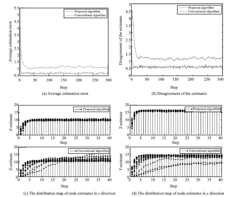
\begin{align*} R_i=\left[\begin{array}{cc}0.8+0.2r_1&0\\0&0.8+0.2r_2\end{array}\right], \end{align*} where $r_1$ and $r_2$ is randomly chosen from the interval [0,1]. The system transition matrix is $A=\left[\begin{array}{cc} 1&0\\0&1\end{array}\right]$ and the output matrix is $H_i=\left[\begin{array}{cc}c_1&0\\0&c_2\end{array}\right]$,where ${{\rm{c}}_{\rm{1}}}$ and ${{\rm{c}}_{\rm{2}}}$ is randomly chosen from the interval $[0.2,0.8]$. The maximum number of iteration is $300$. Here,we choose several nodes that are not mutual neighbors to be attacked. We adjust the observation data according to the size of the attack state and we increase the noise disturbance. Average estimation error and disagreement of estimation are evaluated as follows.

\begin{align*} &E_i(t)=\sqrt{\frac{1}{n}\sum_{i=1}^n(\hat x_i(t)-x_i(t))^{\rm T}(\hat x_i(t)-x_i(t))},\\[0mm] &\psi_i(t)=\sqrt{\frac{1}{n}{\sum_{i=1}^n}(\hat x_i(t)-\hat\varsigma(t))^{\rm T}(\hat x_i(t)-\hat \varsigma(t))}, \end{align*} where $\hat\varsigma(t)=\frac{1}{n}{\sum\nolimits_{i=1}^n}\hat x_i(t)$,$E_i(t)$ evaluates the estimation accuracy,$\psi_i(t)$ evaluates the disagreement of the estimates.

A. Simulation Analysis Under Random Attack

In the random attack model,we assume that 3 randomly selected nodes are under attack. Average estimation error and disagreement of estimation error are illustrated in Figs. 2 (a) and 2 (b), respectively. Figs. 2 (c) and 2 (d) show the distribution map of node state estimates in $x$ direction and $y$ direction.

It can be seen that the proposed algorithm outstandingly improves the performance compared to the conventional one,and it also has a faster convergence of the estimates to the true value of the estimated parameter than the conventional algorithm.

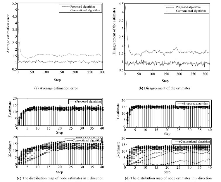
B. Simulation Analysis Under Selective Attack

In the selective attack model,we sort certainty degree of all nodes and select 3 sensor nodes with higher certainty degree to be attacked. Average estimation error and disagreement of the estimates are illustrated in Figs. 3 (a) and 3 (b),respectively. Figs. 3 (c) and 3 (d) show the distribution map of node estimates in $x$ direction and $y$ direction.

From the simulation results,it is obvious that the proposed algorithm outperforms the conventional algorithm,the estimates of the conventional algorithm are somewhat dispersed for a relatively long period. Compared with the random attack model,one selected attacked node has greater impact when some important nodes are under attack. This indicates that in order to improve the estimation performance of the WSN,adding maintenance to such nodes with higher certainty degree is necessary.

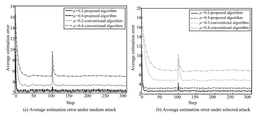
C. Simulation Analysis Under Different Attack Circumstances

As the two attacked models mentioned before,Fig. 4 shows the estimation performance of the two algorithms under different attack circumstances. It is assumed that a sudden jump of node status value occurs when applying Gaussian white noise to some random nodes at time step $t=100$.

From Fig. 4,it can be seen that the attack rate reaches $\mu$ $=$ $0.2$,the proposed algorithm can effectively decrease the error in fusion phase which is caused by the uncertainty. When the attack rate reaches $\mu=0.4$,as the number of attacked nodes increases, the performance of both algorithms deteriorates. The average estimation error variation of the proposed algorithm is less than the conventional algorithm. At time step $t$ $=$ $100$,the simulation results indicate that the conventional algorithm makes the node estimates change greatly while the performance of the proposed algorithm remains fairly stable. It can be shown that when network attack exists,in order to reduce the negative impact,the attacked node information are eliminated by the improved algorithm. We set the attacked node weights to zero in consensus step,then redistribute the attacked node weights to their neighbors,with the aim to dynamically give more importance to the nodes receiving the measurements.~ The~ proposed algorithm improves estimation performance of nodes and estimation accuracy of the WSN.

Ⅵ. CONCLUSION

In this paper,we present a distributed filtering algorithm based on tunable weights under untrustworthy dynamics. Firstly,considering the node location in the network topology,we present an evaluation algorithm to calculate the certainty degree which can be viewed as a metric for a node estimation performance across the sensor network. And then quantitative values are used to optimize consensus protocol which can be viewed as fusion weights to update node status estimates. Based on this,in order to achieve a better estimate of the target state,referring to the idea of load redistribution in complex network theory,we define certainty degree as node load and construct an equation of the weight redistribution. Subsequently,we redistribute the weights of attacked nodes to their neighbors according to certain principles. Simulation results show that whatever attack the sensor network suffers,random attack or selective one,the proposed algorithm not only improves estimation performance,but also provides a strong anti-jamming capability.