 2016, Vol.3


2.the School of Computer Science and Technology, Hubei University of Science and Technology, Wuhan 437100, China;
3.the Institute of Automation, Chinese Academy of Sciences, Beijing 100190, China;
4. Jiangsu Jinling Sci & Tech Group Co., Ltd, Nanjing 210008, China
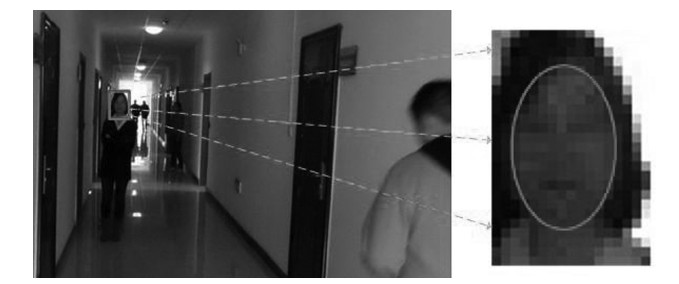
Although face recognition has been studied for nearly a half century and many promising practical face recognition systems have been developed,generally it is assumed that the face region is large enough to contain sufficient information for recognition. With the growing application of surveillance,there is an increasing demand for face recognition especially in very low resolution (VLR) face problem [1] due to the physical limitation of relevant imaging devices. As shown in Fig. 1,when the person is not close enough to the camera,the face region in the scene will be small and therefore limits the performance of established automatic face recognition technology. A potential method to solve the VLR problem is to recover lost high-frequency details in the face images. Therefore, super-resolution (SR) algorithms are employed [2, 3, 4] to reconstruct a high-resolution (HR) face image from a VLR observation.

|
Download:
|
| Fig. 1. Example of VLR face recognition problem. | |
Super-resolutions can be categorized into two classes according to the applied low resolution (LR) images: general SR,which extracts HR images from general LR images,and domain specific SR,which extracts HR images from a restricted class of LR images,such as face or text images. In this paper,we focus on single-frame face image SR,which is also called face hallucination [7] . Face images differ from general images in that they have more regular structure and thus reconstruction constraints in the face domain can be more effective. Because of the self-similarity of the face images,learning-based SR algorithms are always used to enhance the resolution of the face images
The general idea of learning-based approach is to collect a database,learn the statistical correlation between the LR and HR images,and apply it to the input images for reconstruction. For example,Freeman et al. [5] propose a sample-learning SR method based on Markov network,which can be used to learn the relationship between LR and HR images. Hertzmann et al. [6] propose an image analogy SR algorithm based on multi-scale auto regression model.
To improve the quality of the reconstructed human face,Baker and Kanade [7] first propose the term ''face hallucination''. And then Liu et al. [8] propose a two-step modeling method which integrating a global parametric model with a local non-parametric model to hallucinate an HR face image from an LR one. Inspired by Liu's work,many existing works treat face hallucination as a two-step problem. Firstly,a global HR face image is generated which maintains the main characteristics but lacks detailed features. Secondly,a residue image which contains the high-frequency detail information is synthesized and added to the global face image to obtain the final results. For example,in a two-step face hallucination model developed by Zhuang et al. [9] ,locality preserving hallucination algorithm is proposed in the first step instead of PCA to generate the global face image. In the second step,details of the synthesized HR face are then improved by residue compensation,which is inspired by locally linear embedding (LLE). And a global smooth operator is used to further improve the image quality.
Though these methods [8, 9] can improve the quality of the final HR face image to some extent,the computational complexity and the sensitivity to noise cannot be reduced. In [10, 11],face hallucination and recognition are performed directly in Eigenface space. Since Eigenface space is only a subspace generated by applying PCA analysis to the pixel space,its capability of representing a human face is worse than that of the pixel space. By learning the mapping among faces with different resolutions in a unified feature space, Li et al. [12] find that it is possible to carry out LR face recognition without any SR reconstruction preprocessing. Hennings-Yeomans et al. [13] propose an approach for the recognition of LR faces by including an SR model and face features in a regularization framework.
However,the method mentioned above are mainly based on parametric statistical model,and infer an HR face image from an LR one with the nearest feature distance to the tested LR sample. In fact,they are traditional image reconstruction methods to generate HR images directly from LR images. The improvement of reconstruction result is limited because of lack of analysis between training and testing samples. To overcome this problem,different face hallucination methods [14, 15, 16] based on dictionary-learning have been proposed to do something. Yang et al. [14] replace image samples with image patch pairs to generate HR images based on the sparse representation similarity between LR and HR dictionaries. Zeyde et al. [15] further improve this approach by training the observed LR face images. These two methods are based on sparse representation and can be applied to single-frame general image reconstruction problems. Ma et al. [16] propose a face SR method to hallucinate the HR image patch using image patches at the same position of each training image. The position patch constraint is proved to be feasible and robust to facial expression variations and multi-views of face images. This method generates high-quality images and costs less computational time than some former established methods. However,it cannot performance well under noisy environments.
In order to improve the noise resistance performance and the results under complicated situations,we propose a novel face hallucination method based on non-local similarity and multi-scale linear combination (NLS-MLC). Different from most of the established learning-based algorithms,the non-local similarity of face images is considered in the proposed model. For VLR face image recognition, a new method is also proposed based on resolution scale invariant feature (RSIF).
The rest of this paper is organized as follows. In Section Ⅱ,we analysis the attributes of face images,including multi-scale similarity and non-local similarity. Some details of the SR reconstruction are discussed in Section Ⅲ. Face recognition method is proposed in Section Ⅳ. Experimental steps and results are presented in Section Ⅴ,including database and settings, model parameters and result analysis. Section Ⅵ concludes this paper.
Ⅱ. MULTI-SCALE SIMILARITY AND NON-LOCAL SIMILARITY A. Multi-scale SimilarityLearning-based image SR methods are mainly on the basis of two laws of image similarity: 1) large available similar information exists among different images; 2) this similarity can preserve in multi-scale resolutions. This section will discuss the preservation of image multi-scale similarity and its reflection on face hallucination methods.
Image multi-scale similarity preservation can be applied in learning-based face hallucination algorithms because of the similar representation of the tested face image in HR and LR sample spaces. A pair of training face samples with low- and high-resolution is first established respectively,in which the samples in LR are generated from the degradation of the corresponding HR face images (including blurring and down sampling). Because of the similar representation of an input LR image in the LR and HR sample spaces,the expected HR face image can be generated directly from the HR space.
This idea has been employed in recent face hallucination works [14, 15, 16] ,mainly including sparse dictionary representation,which combines sparse representation with multi-scale co-occurrence representation. The common feature of these methods is to achieve face hallucination by capturing the co-occurrence prior [14] from low- and high-resolution patches in multi-scale dictionaries. By generating HR and LR image patch dictionary pairs from image patches,an HR image can be integrated from the HR evaluation of each input LR image patches based on their sparse representation in the LR image patch dictionary. The calculation process is more effective because the avoidance of sparse representation in HR space.
According to sparse signal representation,let $\Phi \in {\bf R}^{n\times K}$ be an overcomplete dictionary of $K$ atoms $(K>n)$. It is assumed that a signal $x\in {\bf R}^n$ can be well represented using a linear combination of a few atoms from dictionary $\Phi $. That is $x$ $=$ $\Phi \alpha _0 $,where $\alpha _0 \in {\bf R}^K$ is a vector with very few ($\ll n)$ nonzero elements. In practice, we might only observe a small set of measurements $y$ of the unknown signal $x$:
| $ \begin{align} \label{eq1} y=Lx=L\Phi \alpha _0, \end{align} $ | (1) |
For single-frame SR reconstruction,the relation between LR image $y_l \in {\bf R}^{N_l }$ and original HR image $x_h \in {\bf R}^{N_h }$ can be described as:
| $ \begin{align} \label{eq2} y_l =HDx_h +v, \end{align} $ | (2) |
where $H:{\bf R}^{N_h }\to {\bf R}^{N_h }$ and $D:{\bf R}^{N_h }\to {\bf R}^{N_l }$ $(N_l <N_h )$ represent blurring filter and down-sampling operator respectively,and $v\sim {\rm N}(0,\sigma ^2I)$ is an additive white Gaussian noise. Given $y_l $,the problem is to find $\tilde {x}\in {\bf R}^{N_h }$ such that $\tilde {x}=x_h $. In order to avoid the complexities caused by the different resolutions between $y_l $ and $x_h $,and in order to simplify the overall reconstruction algorithm,it is assumed that the image $y_l $ is scaled-up by a simple interpolation operator $Q:$ ${\bf R}^{N_l }$ $\to$ ${\bf R}^{N_h }$ (e.g.,bicubic interpolation) that fills-in the missing rows and columns,returning the size of $x_h $. The scaled-up image shall be represented by $x_l $ and it satisfies the equation
| $ \begin{align} \label{eq3} x_l =Qy_l =Q(HDx_h +v)=QHDx_h +Qv=L^{\rm all}x_h +\tilde {v}. \end{align} $ | (3) |
Let $p_h^k =R_k x_h \in {\bf R}^n$ be an arbitrary image patch in an HR image $x_h $,where $R_k :{\bf R}^{N_h }\to {\bf R}^n$ represents the operation of extracting the image patch at position $k$ from the image $x_h $. Non-sampling pixels are not included in $k$ given the influence of interpolation. Assume that $p_h^k \in {\bf R}^n$ can be represented by the sparse linear combination of ${\pmb q}^k\in {\bf R}^m$ in terms of the dictionary $\Phi _h \in {\bf R}^{n\times m}$:
| $ \begin{align} \label{eq4} p_h^k =\Phi _h {\pmb q}^k, \end{align} $ | (4) |
where $\left\| {\pmb q}^k \right\|_0 \ll n$,and $\Phi _h$ is for HR dictionary. Similarly,the corresponding image patch in LR image $x_l $ can be expressed as $p_l^k =R_k x_l $. Therefore (3) can be further presented based on image patches:
| $ \begin{align} \label{eq5} p_l^k =Lp_h^k +\tilde {v}_k, \end{align} $ | (5) |
where $L$ denotes $L^{\rm all}=QHD$,operation based on image patches. Multiply both sides of (4) by $ L$:
| $ \begin{align} \label{eq6} Lp_h^k =L\Phi _h {\rm {\pmb q}}^k. \end{align} $ | (6) |
According to (5) and (6),we have:
| $ \begin{align} \label{eq7} Lp_h^k =L\Phi _h {\rm {\pmb q}}^k=p_l^k -\tilde {v}_k. \end{align} $ | (7) |
Then
| $ \begin{align} \label{eq8} \left\| {p_l^k -L\Phi _h {\rm {\pmb q}}^k} \right\|_2 \le \varepsilon, \end{align} $ | (8) |
where the value of $\varepsilon $ is determined by the energy of the noise $v$. Equation (5) is applied to each atom pair in HR dictionary $\Phi _h $ and LR dictionary $\Phi _l $,and then we will have $\Phi _l =L\Phi _h $ under certain fault tolerant error $\varepsilon $. Equation (8) can be rewritten as
| $ \begin{align} \label{eq9} \left\| {p_l^k -\Phi _l {\rm {\pmb q}}^k} \right\|_2 \le \varepsilon. \end{align} $ | (9) |
Comparing (4) with (9),we will find the similar sparse representation of high- and low-resolution image patch pair $p_h^k $ and $p_l^k $ in terms of high- and low-resolution dictionaries $\Phi _h $ and $\Phi _l $. Therefore,the sparse representation coefficient ${\rm { \hat {\pmb q}}}^k$ can be calculated by (9) with regard to a specific image patch,and then ${{\pmb {q}}}^k$ is applied to (4) to generate the evaluation of HR image patch and finally the entire HR image is obtained.
B. Non-local SimilarityAccording to Markov random theory,a pixel value is completely determined by pixels in the field around while independent of other pixels far away. Generally,many image processing and signal processing methods are based on this similarity. A typical example is the neighborhood filter method. The neighborhood system ${\cal N}=\left\{ {{\cal N}_i } \right\}_{i\in I} $ of image $I$ is a subset of the image pixel set. Given $i\in I$,if $j\in{\cal N}_i\Rightarrow$ $i$ $\in$ ${\cal N}_j $,then ${\cal N}_i $ is the neighborhood or similar window of pixel $i$,defined as $\tilde {{\cal N}}_i ={\cal N}_i \backslash \left\{ i \right\}$.
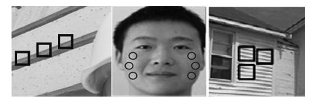
However,neighborhood similarity cannot reflect the essential similarity of natural images. In fact,image similarity not only exists in local pixels but also in non-local regions. For example, similar pixels of a certain pixel can be found in the whole image pixel space instead of its neighborhood. Generally,an image will contain sufficient repetitive structure as shown in the square and circle windows in Fig. 2 and therefore result in image information redundancy. This phenomenon can be understood easily when these pixels are close to each other,and is called local similarity assumption. The idea can be extended to any position in the image. Based on the concept of neighborhood,we define the non-local region of pixel $i$ is a set of pixels $\{j\}$ in the image,$j$ satisfies the condition that the neighborhood of $j$ resembles that of pixel $i$. All pixels in the non-local region (for example,pixel $j)$ will contain similar information for pixel $i$ and therefore can be used to predict the pixel value of $i$.

|
Download:
|
| Fig. 2. Image non-local similarity. | |
As discussed above,face image as a specific image possesses multi-scale similarity and non-local similarity. Based on these properties,we propose a novel face hallucination method based on non-local similarity and multi-scale linear combination (NLS-MLC). Meanwhile,a new VLR face recognition is also proposed based on resolution scale invariant feature (RSIF).
Ⅲ. NLS-MLC FACE HALLUCINATION A. Multi-scale Linear Combination ConsistencyLet $I^H$ be an arbitrary HR image,and the corresponding LR image $I^L$ can be generated by the degradation of $I^H$:
| $ \begin{align} \label{eq10} I^L=DHI^H+N, \end{align} $ | (10) |
where $I^H$ and $I^L$ are column vectors,$N$ is the random Gaussian noise evenly distributed in the image,$D$ and $H$ denote the down-sampling and blurring operator respectively,and the down-sampling factor is $s$. Divide these images into patches:
| $ \begin{align} \label{eq11} P_{i,j} (I^L)&=P_{i,j} (DHI^H)+P_{i,j} (N)\notag\\ &=D_P H_P P_{k,l} (I^H)+P_{i,j} (N), \end{align} $ | (11) |
where $P_{i,j} (I^L)$ represents an image patch of $q\times q$ centered on the $(i,j)$ pixel from LR images. Let $I^L (i,j)$ be a column vector of $P_{i,j} (I^L)$ and $(i,j)~{\rm s.t.}~(si,sj)=(k,l)$. Because of the uniform distribution of noise in the images,(11) can be rewritten as:
| $ \begin{align} \label{eq12} I^L (i,j)=D_P H_P I^H(k,l)+n. \end{align} $ | (12) |
In the training phase,we generate an HR and LR image patch dictionary pair. Assuming that there are $M$ images in HR samples $I_m^H$ $(m=1,\ldots ,M)$,the corresponding LR samples can be represented as $I_m^L$ $(m=1,\ldots ,M)$. Each HR or LR image is divided into image patches with overlap to form HR and LR image patch sets. They are $S^H=\{I_m^H (k,l)\vert m=1,\ldots ,M;(k,l)\in \Omega ^H\}$ and $S^L=$ $\{I_m^L (i,j)\vert m$ $=$ $1,$ $\ldots ,$ $M;$ $(i,j)\in \Omega ^L\}$,where $\Omega ^H$ and $\Omega ^L$ represent the position ranges of the image patches.
Denote $T,T^H,T^L$ as integer variables,and let $T^H=\| {S^H} \|$, $T^L=\| {S^L} \|$,where $\|\cdot\|$ denotes the set cardinality. Evidently $T=T^H=T^L$. Equation (12) can tell the relation between the corresponding HR and LR patches:
| $ \begin{align} \label{eq13} I_m^L (i,j)=D_P H_P I_m^H (k,l)+n. \end{align} $ | (13) |
Two coupled dictionaries are generated respectively: $A^H=$ $[I^H (1);I^H (2);\ldots ;I^H (T)]$ for HR image patches and $A^L=$ $[ I^L (1);I^L (2);\ldots ;I^L (T)]$ for LR image patches with a one-to-one correlation shown in (13). Each column in the dictionary is a vector formed by pixels in an image patch. For example,the $t$-th column in $A^L$ can be represented as $I^L (t)$ $=$ $A^Le_t $,$e_t $ is a column vector with one for the $t$-th element and zeros for the other elements. We have:
| $ \begin{align} \label{eq14} A^L=D_P H_P A^H+V, \end{align} $ | (14) |
where $V=[n;n;\ldots]$,and is the same size as $A^L$.
Let $Y$ be the testing LR face image,and we assume that $Y$ is generated from an unknown HR image $X$ by the degradation processing in (10),that is:
| $ \begin{align} \label{eq15} Y=DHX+N. \end{align} $ | (15) |
We divide $Y$ into image patches. The image patch $Y(i,j)$ centered at $(i,j)$ can be represented as:
| $ \begin{align} \label{eq16} Y(i,j)=D_P H_P X(k,l)+n. \end{align} $ | (16) |
We define the non-local similar image patch set of $Y(i,j)$ in $A^L$ as $\Phi _{i,j}^L =\{I_m^L (i',j')\vert m=1,\ldots ,M;(i',j')\in N_r^L (i,j)\}$ $=$ $A^LF_{i,j} $,where $N_r^L (i,j)$ is the non-local region in the LR image centered at $(i,j)$ and with a radius of $r$. $F_{i,j} $ is a matrix with $\| {\Phi _{i,j}^L } \|$ elements of all $e_t $,$F_{i,j}=[{\ldots ;e_{t_{(i',j';m)} } ;\ldots }]$,and $t(i',j';m)$ denotes the serial number of image patch in the $m$-th image centered at $(i',j')$ of $A^L$.
According to the linear combination theory,$Y(i,j)$ can be represented by the linear combination of its non-local similar image patches.
| $ \begin{align} \label{eq17} Y(i,j)=\Phi _{i,j}^L W^L=A^LF_{i,j} W^L, \end{align} $ | (17) |
where $W^L$ is the coefficient matrix and its size is determined by $\left\| {\Phi _{i,j}^L } \right\|$.
Similarly,image patches in HR image $X$ can be represented by the linear combination of its non-local similar patches:
| $ \begin{align} \label{eq18} X(k,l)=\Phi _{k,l}^H W^H=A^HF_{k,l} W^H. \end{align} $ | (18) |
Because of the corresponding relation of HR and LR image patches, we have $F_{k,l} =F_{i,j} $. By substituting (18) for (16),we get:
| $ \begin{align} \label{eq19} Y(i,j)=D_P H_P A^HF_{i,j} W^H+n. \end{align} $ | (19) |
We combine (19) and (14) to get:
| $ \begin{align} \label{eq20} Y(i,j)&=(A^L-V)F_{i,j} W^H+n\nonumber\\ &=A^LF_{i,j} W^H-VF_{i,j} W^H+n. \end{align} $ | (20) |
Because $V=[n;n;\ldots]$,we can further have $VF_{i,j} W^H=n$. Equation (20) can be simplified as:
| $ \begin{align} \label{eq21} Y(i,j)=A^LF_{i,j} W^H. \end{align} $ | (21) |
Comparing (17) to (21),it is evident that $W^H=W^L$. Then we can conclude that the linear combination of an image patch in terms of its non-local similar patches is consistent in HR and LR spaces. Therefore we have tested the multi-scale linear combination consistency. Notably,when the degradation process of the testing image and the training image are the same,the error between $W^L$ and $W^H$ is theoretically zero regardless of the noise energy. However,the existing methods [14, 15, 16] are all sensitive to noise. Later we will show that our proposed method is more robust to noise and costs less computational time than most existing methods.
By integrating the overlapping image patches generated through the linear combination process,we will have the final HR version $\hat {X}$ of the input LR image,that is:
| $ \begin{align} \label{eq22} \hat {X}(k,l)=A^HF_{k,l} \hat {W}^H=A^HF_{k,l} W^L. \end{align} $ | (22) |
As discussed above,this paper proposes a novel face hallucination method based on non-local similarity and multi-scale linear combination (NLS-MLC). NLS-MLC contains two phases: the training phase and the reconstructing phase. During the training phase,HR and LR image patch dictionary pair is learnt from training face image samples. During the reconstructing phase,the output HR image is generated based on the same linear representation of the tested image with respect to the dictionary pair. Detailed steps of this algorithm are discussed below.
1) The training phase:
a) Determine the degradation process,including the noise variance and fuzzy parameters,based on the observed LR input image and the HR image samples.
b) Generate the corresponding LR image samples by degrading each HR face image through the same degradation process.
c) Each HR or LR image is divided into a set of small corresponding image patches with overlap,the patch size of the HR image is $bs\times bs$ and the LR image $b\times b$,where $s$ is the down-sampling factor.
2) The reconstructing phase:
a) Divide the input LR image into $b\times b$ patches with overlap in the same way as processing training LR samples.
b) We apply gray correlation analysis (GCA) [19] to measure the similarity among image patches for searching non-local similar patches. As a significant branch of gray system theory,GCA can unveil the uncertain correlation between two things and has been widely used to predict the unknown from available information. The gray correlation is computed based on geometric shapes of a curve sequence. While a face image contains much high-dimensional information and pixel values of each image patch can be represented as a curve after vectorization. Therefore GCA is theoretically feasible to solve the non-local similar patch searching problem. Some basic steps of GCA are discussed below.
ⅰ) Preprocess the original data $X=\left\{ {X(k)\vert k=1,2,\ldots, n} \right\}$. There are two common ways:
Initialization: ${X}'(k)={X(k)}/ {X(1)}$,$k=1,2,\ldots ,n$;
Equalization: ${X}'(k)={X(k)}/ {\overline {X}(k) }$,where $\overline {X}(k) =1 / n{\sum\nolimits_{k=1}^n {X(k)} }$.
ⅱ) Define the basic sequence and the subsequence respectively:
Basic sequence: $X_0 =\left\{ {X_0 (k)\vert k=1,2,\ldots ,n} \right\}; $
Subsequence: $Xi=\left\{ {X_i (k)\vert k=1,2,\ldots,n} \right\}$,$i=1,2,$ $\ldots ,$ $m$.
ⅲ) Calculate the correlation coefficient of $X_i (k)$ and $X_0 (k)$ at each point,Deng interrelatedness is calculated here:
| $ \begin{align} \label{eq23}& \xi _i (k)=\notag\\ &{\small \quad\frac{\mathop {\rm min}\limits_i \mathop {\rm min}\limits_k \left| {X_0 (k)-X_i (k)} \right|+\rho \mathop {\rm max}\limits_i \mathop {\rm max}\limits_k \left| {X_0 (k)-X_i (k)} \right|}{\left| {X_0 (k)-X_i (k)} \right|+\rho \mathop {\rm max}\limits_i \mathop {\rm max}\limits_k \left| {X_0 (k)-X_i (k)} \right|}}. \end{align} $ | (23) |
ⅳ) Calculate the final correlation:
| $ \begin{align} \label{eq24} \gamma _i =\frac{1}{n}\sum\limits_{k=1}^n {\xi _i (k)}. \end{align} $ | (24) |
3) For every patch in the input image,the normalized weights of each similar patch are calculated:
| $ \begin{align} &\label{eq25} \tilde {w}(i',j',i,j;s)=\frac{{w(i',j',i,j;s)}} {{\sum\limits_{(i',j')\in N(i,j),1\le s\le M} {w(i',j',i,j;s)} }},\\ \end{align} $ | (25) |
| $ \begin{align} &\label{eq26} w(i',j',i,j;s)=\exp \left\{ {-\frac{\left\| {P_{i',j'} y_s -P_{i,j} y_t } \right\|_2^2 }{2\alpha ^2 }} \right\}\cdot f(d), \end{align} $ | (26) |
where $y_t $ and $y_s $ denote the LR testing sample and the LR training sample respectively,$P_{i,j} $ is a $b\times b$ patch extracted from the input image and centered at pixel $(i,j)$ to be estimated,$(i',j')$ is the non-local similar pixel of $(i,j)$ in the LR image,${{\pmb d}}$ represents the distance between these two pixels,$f$ is a monotonic non-increasing function and is Gaussian function here $f(d)=\rho {\rm e}^{\frac{d^2} {\sigma^2}}$,and $\alpha $ is determined by the estimated value of standard deviation of the noise.
4) Reconstruct the HR version of the input LR image patch $P_{i,j} x_t $:
| $ \begin{align} \label{eq27} P_{k,l} x_t =\sum\limits_{(i',j')\in N(i,j),1\le s\le M} {P_{k',l'} x_s \cdot \tilde {w}(k',l',k,l;s)}. \end{align} $ | (27) |
Pixel $(k',l')$ is the corresponding pixel of $(i',j')$ in the HR image patches. The weight convex is the same as in the LR image patches,that is:
| $ \begin{align} \label{eq28} \tilde {w}(k',l',k,l;s)=\tilde {w}(i',j',i,j;s). \end{align} $ | (28) |
Then (27) can be rewritten as
| $ \begin{align} \label{eq29} P_{k,l} x_t =\sum\limits_{(i',j')\in N(i,j),1\le s\le M} {P_{k',l'} x_s \cdot \tilde {w}(i',j',i,j;s)}. \end{align} $ | (29) |
5) Integrate the overlapped image patches generated in the HR space to obtain the final HR image evaluation of the input one. The final value of each pixel is calculated by averaging several evaluation values in different image patches.
Ⅳ. RSIF FACE RECOGNITIONThe details of facial features are crucial for face recognition in surveillance video,but the resolution of a face image is normally low,causing some losses of facial features. Usually two approaches can be applied to solve this problem. One is to enhance the quality of imaging equipment to obtain HR face images,but it is limited by cost and craftsmanship. The other one is to recover the loss information in the LR image by a SR algorithm. Many such algorithms [10, 17, 18] have been proposed in the last decade and have solved relevant problems to some extent. With regard to VLR face recognition,existing algorithms can be applied to the HR image reconstructed by our NLS-MLC method. In order to improve the recognition performance of VLR face images, this paper propose a novel face recognition approach based on resolution scale invariant feature (RSIF). Section Ⅲ-A proves that the linear combination coefficients of non-local image patches are the same regardless of image resolution. Therefore these coefficients can be used as facial features for recognition. RSIF can avoid the process of SR face reconstruction and is robust to resolution variations. It consists of three steps: data preprocessing,coefficients calculation and recognition.
1) Data preprocessing
Firstly,manually align and crop face images to the same size. Secondly,generate the corresponding LR face image space from degradation of the HR images. Thirdly,divide these images into patches and search their non-local similarity patches.
2) Coefficients calculation
Assume that image patch $Y(i,j)$ can be represented as the linear combination of its similar image patches:
| $ \begin{align} \label{eq30} Y(i,j)=\Phi _{i,j}^L W^L, \end{align} $ | (30) |
where $\Phi _{i,j}^L $ is the set of non-local similar image patches in the LR dictionary,rewritten as $\Phi _m^L, m=1,2,\ldots,M$ for the sake of clearness,$M$ is the number of similar patches,$W^L$ is the weight matrix and the weight value $w_m^L $ denotes the contribution of each similar non-local image patch to the corresponding input image patch. So (30) can be rewritten as:
| $ \begin{align} \label{eq31} Y(i,j)=\sum\limits_{m=1}^M {w_m^L \Phi _m^L (i,j)+e}, \end{align} $ | (31) |
where $e$ is the reconstruction error. Calculating the coefficients $W^L$ means minimizing the reconstruction error $e$:
| $ \begin{align} \label{eq32} W^L=\mathop {\arg }~\mathop {\min }\limits_{w_m } \left\| {Y(i,j)-\sum\limits_{m=1}^M {w_m^L \Phi _m^L (i,j)} } \right\|^2. \end{align} $ | (32) |
Equation (32) is a constrained least square problem. The constraint condition is $\sum\nolimits_{{m=1}}^{M} {w_m^L =1} $. The solving methods are time-consuming such as sparse representation [14] or exist unreliable solution problem in Ma's method [16] . In order to address this problem,this paper employs (23) and (24) to calculate weight coefficients. Experiments in the next section show that this method is simple,rapid and robust.
3) Recognition
Since we represent a face by a set of linear combination coefficients and these coefficients are concatenated to form a vector. To compare two faces $a_1 $ and $a_2 $ in a vector space,in this paper,we use the nearest neighbor classifier with the distance measure being the cosine of the angle between these two vectors:
| $ \begin{align} \label{eq33} d=\frac{\langle a_1 ,a_2 \rangle}{\left\| {a_1 } \right\|\left\| {a_2 } \right\|}. \end{align} $ | (33) |
For identification,any input face is reported to be the one in the database which has the largest $d$ between the two. For verification,two faces are claimed to be of the same individual if $d$ between them is larger than a predefined threshold. For each query image,the score data for each subject from each patch is passed to the combiner. Since the score data has been normalized so that it approximates a probability,a number of simple classifier combination strategies can be employed. In our implementation,we employ the sum-rule [27] .
Ⅴ. EXPERIMENTS AND ANALYSIS A. Experiment Ⅰ: Visual QualityPublic face database CAS-PEAL-R1 [20] is selected for this experiment. Face images in this database contain variations in expression,pose,occlusion and age. In this paper,a subset that consists of 1000 frontal view images (one per person) with normal expression or pose is used. These images are manually aligned and cropped to the resolution of 128 $\times$ 96 to make up the HR face image samples. Four experiments are conducted to evaluate the algorithm,including frontal face image reconstruction and noise resistance analysis,facial expression reconstruction,pose variation reconstruction,and real world image reconstruction.
To show that the algorithm is independent of training samples,we randomly sample 500 face images from the 1000 individuals to form the HR face image space in each experiment. The corresponding LR face image space with the size of 32 $\times$ 24 is generated through degrading HR images. We apply the method in Section Ⅲ.B to divide these images into patches and form an image patch dictionary pair with the same number of HR and LR image patches respectively. Finally we perform our algorithm to recover a HR image of 128 $\times $ 96 from the LR image of 32 $\times $ 24. The size of LR image patch is 3 $\times $ 3 and HR image patch is 12 $\times $ 12 in these experiments.
1) Frontal face images
The purpose of this experiment is to test the independence of training samples and analyze the impact of noise. We compare our results with Ma's results [16] . This experiment includes two cases: i) the testing face image is in the training database; ⅱ) the testing face image is not in the training database,and we analyze the impact of noise in the second case.
a) Testing sample in the training database:
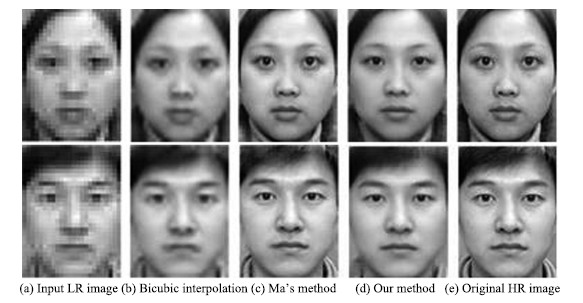
Fig. 3 illustrates two examples of hallucinating face images using traditional bicubic interpolation,Ma's method and our NLS-MLC method. The results show that our method and Ma's method are better than the traditional bicubic interpolation from visual perspective.

|
Download:
|
| Fig. 3. Reconstruction results when the testing image is in the training database. | |
b) Testing sample not in the training database:
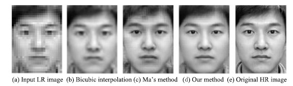
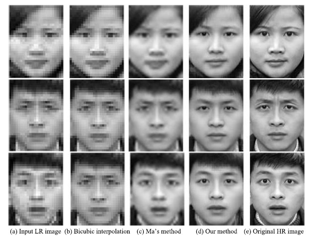
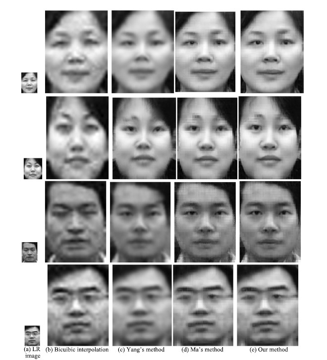
Without noise: Fig. 4 shows the face hallucination results when the testing image is not in the training database. Comparing with Fig. 3,we can conclude that our method is nearly the same whether the testing sample is in or is not in the training set,while the performance of Ma's method decreases in the second case. Therefore, our method is more independent to the training samples compared to Ma's method.

|
Download:
|
| Fig. 4. Reconstruction results when the testing image is not in the training database and without noise. | |
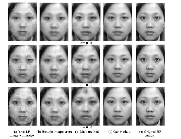
With noise: In order to analyze the impact of noise,zero mean Gaussian noise is added to the LR input face image in Fig. 5. Each row represents the reconstruction results under different noise intensity. With the increase of noise intensity,face hallucination result quality decreases dramatically,however only our method is robust to noise.

|
Download:
|
| Fig. 5. Reconstruction results when the testing image is not in the training database and with noise. | |
2) Face images with expression variations
The purpose of this experiment is to test the feasibility of our method to reconstruct face images with expression variations. We study the hallucination performance with test set containing face images with expression variations and training set containing face images without expression variations. Some representative examples are shown in Fig. 6. The results indicate that our method is also applicable to input face image with expression variations.

|
Download:
|
| Fig. 6. Reconstruction results with expression variations. | |
3) Face images with pose variations
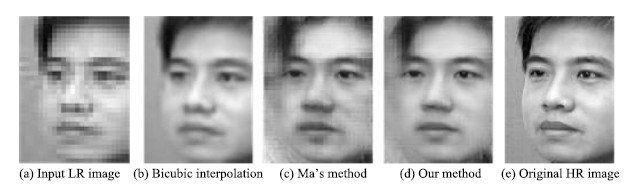
The purpose of this experiment is to test the feasibility of our method to reconstruct face images with pose variations. We study the hallucination performance with test set containing face images with pose variations and training set containing face images without pose variations. The result shown in Fig. 7 indicates that our method is better than Ma's method concerning pose variations.

|
Download:
|
| Fig. 7. Reconstruction results with expression variations. | |
4) Real world images
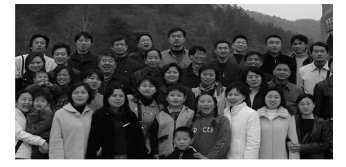
A real world image shown in Fig. 8 is used to further verify our method. Some representative reconstruction results are shown in Fig. 9. The resolution of the face images are enhanced by our method.

|
Download:
|
| Fig. 8. Test image. | |

|
Download:
|
| Fig. 9. Reconstruction results in real world image. | |
5) Objective measure index in experiment
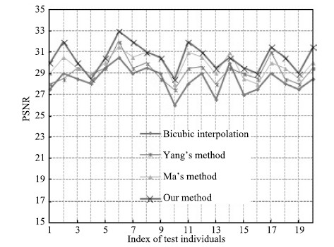
To quantify the results from the ground truth data,we also computed the peak signal-to-noise ratio (PSNR) for each method. All the results are shown in Fig. 10. It can been see that our method has the highest PSNR values compared to the values of other methods for all test faces.

|
Download:
|
| Fig. 10. PSNR values of the hallucinated results from three different methods. | |
Sample dictionary pair can be prepared offline because it has been proved that our proposed method is independent of face image samples. Therefore we can reduce the computational time because only reconstructing is computed online. Except for the third experiment, the average time of the reconstruction phase in our experiments is 0.316 s using PC with Intel Core (TM) 2 Quad CPU 8300,2.5 GHz and 2 G memory,and using Matlab 7.1. However the reconstruction time of Ma's method is 40.75 seconds with the same experiment environment.
B. Experiment Ⅱ: Recognition PerformanceWe would like to further evaluate the performance of the proposed algorithm in terms of recognition accuracy. The experimental results are organized as follows: 1) reports the performance of NLS-MLC face hallucination and other SR reconstruction methods on the FRGC V2.0 database using face recognition algorithms,namely,PCA+1NN, KPCA+1NN,KLDA+1NN,PCA+SVM; 2) studies the performance of our proposed RSIF face recognition method on testing images with different resolutions.
1) NLS-MLC
Databases and settings: In this experiment,two public face image databases are used,FRGC V2.0 [21] and CAS-PEAL. For FRGC V2.0 database,we select ten images per person with a near-frontal view and mild expression variations. The individuals with less than ten applicable images are discarded. Finally a subset of 311 individuals is selected for our experiments. For the CAS-PEAL database,we select eleven images per person with expression and pose variations. For each person,six images are used as a gallery set while the rest five images are used as a probe set. Details of the database settings are given in Table Ⅰ,$N_{C}$ denotes the number of individuals,$N_{G}$ denotes the number of training images per person and $N_{P}$ denotes the number of test images per person. As for FRGC V2.0 database,it is noted that the training set is the same as the gallery set,whereas the testing set is non-overlapped with the training set.
|
|
Table Ⅰ DATABASE SETTINGS FOR EXPERIMENT Ⅱ |
Results and analysis: This experiment studies the recognition performance of our NLS-MLC algorithm on FRGC V2.0. To evaluate the performance of the proposed method on a face recognition system,we carry out the experiments using the reconstructed HR images with some existing face recognition algorithms,i.e.,PCA+1NN,KPCA+1NN, PCA+SVM and KLDA+1NN. The VLR and HR images are used as benchmark performance,and four existing SR algorithms (EF [22] , KF [23] ,PF [16] ,DSR [1] ) are selected for comparison.
For the PCA+1NN face recognition algorithm,PCA is used to extract the eigenfaces as the feature for the 1NN classifier. The results are plotted in Fig. 11. We can see that the gap between recognition accuracy of VLR images and HR images is around 20 %. Existing SR algorithms such as EF and DSR can slightly improve the recognition accuracy of VLR images whereas KF and PF even worsen the performance to some extent. However our NLS-MLC method can improve the performance significantly. We use the same classifier but change the feature extractor from PCA to kernel PCA (KPCA) and repeat the experiments. The results are shown in Fig. 12. Similar conclusions are obtained. That is,the recognition accuracy of our method approximates that of the original HR images.

|
Download:
|
| Fig. 11. Recognition results on FRGC V2.0 with PCA+1NN face recognition engine. | |

|
Download:
|
| Fig. 12. Recognition results on FRGC V2.0 with KPCA+1NN face recognition engine. | |
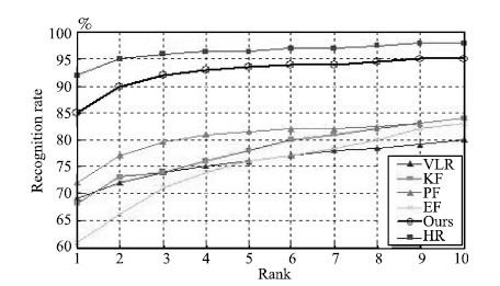
For further evaluation,we conduct more experiments with discriminative face recognition algorithms,such as KLDA+ 1NN [24] and PCA+SVM. For KLDA,Gaussian radial basis function is used as the kernel function. For SVM,we use the linear kernel as the kernel function. And the results are plotted in Figs. 13 and 14. The recognition accuracy on VLR images is around 20 % lower than that of the HR images. However,our method has around 10 % improvement than the HR images while the performance of other SR algorithms is either slightly better or even lower than that of VLR images.

|
Download:
|
| Fig. 13. Recognition results on FRGC V2.0 with PCA+SVM face recognition engine. | |
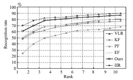

|
Download:
|
| Fig. 14. Recognition results on FRGC V2.0 with KLDA+1NN face recognition engine. | |
2) RSIF
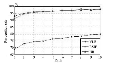
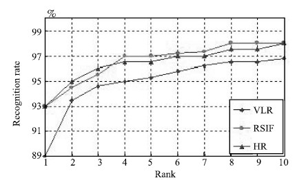
In this experiment,we evaluate the performance of the proposed RSIF algorithm on images with different resolutions. In addition to our method (RSIF),KLDA was used to extract the feature for the 1NN classifier. For FRGC V2.0 database, images of 7 $\times$ 6,14 $\times$ 12,and 28 $\times$ 24 are used as testing LR set,and HR images of 56 $\times$ 48 are used as training set. For the CAS-PEAL database,images of 8 $\times$ 6,16 $\times$ 12,32 $\times$ 24,and 64 $\times$ 48 are used as testing LR set,and HR images of 128 $\times$ 96 are used as training set. Other settings are the same as 1).
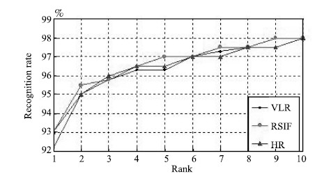
The results are shown in Figs. 15-17. The proposed method can improve the performances for all of the three resolutions. For images of 7 $\times$ 6,the recognition rate of RSIF approximates that of the original HR images. For images of 14 $\times$ 12,and 28 $\times$ 24,the performances of RSIF are even better than that of the original HR images. Moreover,the recognition rates of RSIF on three different resolutions are nearly the same. This means that RSIF is robust to resolution variations and can be used to solve VLR face recognition problem.

|
Download:
|
| Fig. 15. Recognition results of 7 $\times$ 6 LR images. | |

|
Download:
|
| Fig. 16. Recognition results of 14 $\times$ 12 LR images. | |

|
Download:
|
| Fig. 17. Recognition results of 28 $\times$ 24 LR images. | |
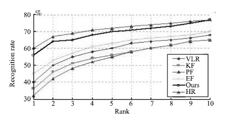
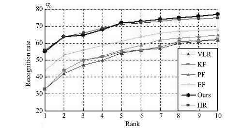
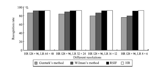
We further conduct our experiments on CAS-PEAL face image database. The purpose of this experiment is to compare the proposed RSIF method with some VLR face recognition algorithms,such as Gunturk's method [8] ,Wilman's method [1] . Face images with different resolutions are used for experiments. The results are shown in Fig. 18. We can conclude that RSIF face recognition method is better than the other methods used in this experiment.

|
Download:
|
| Fig. 18. Recognition results of face images with different resolutions using different face recognition algorithms. | |
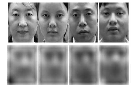
It is obvious that,when a face image is of size 8 $\times$ 6,it does not look like a human face. As shown in Fig. 19,the face images on top are of size 128 $\times$ 96,and the face images on bottom are of size 8 $\times$ 6. The faces cannot be recognized by human eyes,but they can still be recognized by machine using our algorithm. Inspired by the face recognition methods of Eigenfaces and Fisherfaces,the multi-scale linear combination consistency and non-local similarity characteristics are used for face SR and recognition,which can solve the VLR problem. However,it is important to note that the VLR images are generated just by down-sampling and blurring operator,and it is a little different from real VLR face images.

|
Download:
|
| Fig. 19. The HR and LR face images. | |
In this paper,non-local similarity and multi-scale linear combination (NLS-MLC) is defined and proved to be consistent in images with different resolutions. Therefore it can be applied in SR face reconstruction. We propose a novel dictionary learning method for face hallucination based on NLS-MLC. Experimental results have shown that the proposed algorithm is robust to noise, expression and pose variations. Based on the linear combination consistency,a novel face recognition method is proposed based on RSIF to enhance the performance of VLR face recognition. Experimental results have shown that the performance of this new algorithm is better than some existing face recognition methods and is robust to resolution variations.
| [1] | Zou W W W, Yuen P C. Very low resolution face recognition problem. IEEE Transactions on Image Processing, 2012, 21(1): 327-340 |
| [2] | Yang J, Huang T. Image super-resolution: historical overview and future challenges. Super-Resolution Imaging. Boca Raton, FL: CRC Press, 2010. |
| [3] | Park S C, Park M K, Kang M G. Super-resolution image reconstruction: a technical overview. IEEE Signal Processing Magazine, 2003, 20(3): 21 -36 |
| [4] | van Ouwerkerk J. Image super-resolution survey. Image and Vision Computing, 2006, 24(10): 1039-1052 |
| [5] | Freeman W T, Jones T R, Pasztor E C. Example-based super-resolution. IEEE Computer Graphics and Applications, 2002, 22(2): 56-65 |
| [6] | Hertzmann A, Jacobs C E, Oliver N, Curless B, Salesin D H. Image analogies. In: Proceedings of the 28th Annual Conference on Computer Graphics and Interactive Techniques. Los Angeles, California: ACM, 2001. 327-340 |
| [7] | Baker S, Kanade T. Hallucinating faces. In: Proceedings of the 4th IEEE International Conferences on Automatic Face and Gesture Recognition. Grenoble, France: IEEE Press, 2000. 83-88 |
| [8] | Liu C, Shum H Y, Zhang C S. A two-step approach to hallucinating faces: global parametric model and local nonparametric model. In: Proceedings of the 2001 IEEE Computer Society Conference on Computer Vision and Pattern Recognition. Kauai, HI, USA: IEEE, 2001. Ⅰ-192-Ⅰ- 198 |
| [9] | Su C Y, Zhuang Y T, Huang L, Wu F. Steerable pyramid-based face hallucination. Pattern Recognition, 2005, 38(6): 813-824 |
| [10] | Gunturk B K, Batur A Z, Altunbasak Y, Hayes M H, Mersereau R M. Eigenface-domain super-resolution for face recognition. IEEE Transactions on Image Processing, 2003, 12(5): 597-606 |
| [11] | Wan Z F, Miao Z J. Feature-based super-resolution for face recognition. In: Proceedings of the 2008 IEEE International Conference on Multimedia and Exposition. Hannover, Germany: IEEE, 2008. 1569-1572 |
| [12] | Li B, Chang H, Shan S G, Chen X L. Low-resolution face recognition via coupled locality preserving mappings. IEEE Signal Processing Letters, 2010, 17(1): 20-23 |
| [13] | Hennings-Yeomans P H, Baker S, Kumar B V K V. Simultaneous superresolution and feature extraction for recognition of low-resolution faces. In: Proceedings of the 2008 IEEE Conference on Computer Vision and Pattern Recognition. Anchorage, AK: IEEE, 2008. 1-8 |
| [14] | Yang J C, Wright J, Huang T S, Ma Y. Image super-resolution via sparse representation. IEEE Transactions on Image Processing, 2010, 19(11): 2861-2873 |
| [15] | Zeyde R, Elad M, Protter M. On single image scale-up using sparserepresentations. In: Proceedings of the 7th International Conference, Lecture Notes in Computer Science. Avignon, France: Springer, 2012. 711-730 |
| [16] | Ma X, Zhang J P, Qi C. Hallucinating face by position-patch. Pattern Recognition, 2010, 43(6): 2224-2236 |
| [17] | Huang H, He H T. Super-resolution method for face recognition using nonlinear mappings on coherent features. IEEE Transactions on Neural Networks, 2011, 22(1): 121-130 |
| [18] | Jiang J, Hu R, Han Z, Huang K. Graph discriminant analysis on multi-manifold (GDAMM): a novel super-resolution method for face recognition. In: Proceedings of the 2012 IEEE International Conference on Image Processing. Orlando, FL: IEEE, 2012. 1465-1468 |
| [19] | Liu S F, Lin Y. Grey Information: Theory and Practical Applications. London: Springer-Verlag, 2005. |
| [20] | Gao W, Cao B, Shan S G, Chen X L, Zhou D L, Zhang X H, Zhao D B. The CAS-PEAL large-scale Chinese face database and baseline evaluations. IEEE Transactions on Systems, Man, and Cybernetics, Part A: Systems and Humans, 2008, 38(1): 149-161 |
| [21] | Phillips P J, Flynn P J, Scruggs T, Bowyer K W, Chang J, Hoffman K, Marques J, Min J, Worek W. Overview of the face recognition grand challenge. In: Proceedings of the 2005 IEEE Computer Society Conference on Computer Vision and Pattern Recognition. San Diego, CA, USA: IEEE, 2005. 947-954 |
| [22] | Wang X G, Tang X O. Hallucinating face by eigentransformation. IEEE Transactions on Systems, Man, and Cybernetics, Part C: Applications and Reviews, 2005 35(3): 425-434 |
| [23] | Chakrabarti A, Rajagopalan A N, Chellappa R. Super-resolution of face images using kernel PCA-based prior. IEEE Transactions on Multimedia, 2007, 9(4): 888-892 |
| [24] | Liu C J. Capitalize on dimensionality increasing techniques for improving face recognition grand challenge performance. IEEE Transactions on Pattern Analysis and Machine Intelligence, 2006, 28(5): 725-737 |
| [25] | Donoho D L. Compressed sensing. IEEE Transactions on Information Theory, 2006, 52(4): 1289-1306 |
| [26] | Rauhut H, Schnass K, Vandergheynst P. Compressed sensing and redundant dictionaries. IEEE Transactions on Information Theory, 2008, 54(5): 2210-2219 |
| [27] | Kittler J, Hatef M, Duin R P W, Matas J. On combining classifiers. IEEE Transactions on Pattern Analysis and Machine Intelligence, 1998, 20(3): 226-239 |