 2016, Vol.3


Face recognition techniques are mainly used to match unknown face images with an identified set of images for addressing security problems. As surveillance systems in wide range of public places are increasing,the demand for face recognition techniques for security and surveillance applications is increasing. Though classic face recognition approaches such as [1, 2, 3, 4] perform very well,their successes are confined to the conditions of strictly controlled scenarios,which are unrealistic in wide range of real applications. Real-life face recognition systems usually suffer from poor resolution,illumination and pose variation conditions,which adversely degrade the performance of most existing face recognition approaches [5] . Therefore,it is necessary to consider the issue of robust face recognition systems which can jointly handle poor resolution,illumination and pose variations.
During the past decades,research in the field of face recognition has been mainly focused on recognizing faces across variations in illumination and pose [6, 7, 8] . That is because they are still considered as major challenges encountered by current face recognition techniques. There is a recent trend towards addressing the problem of poor resolution face image recognition [9, 10, 11, 12, 13, 14] ,as the poor resolution face images are common in real life. For example,when subjects are far from cameras without any restriction, the face regions are very small or of poor quality,which causes low-resolution (LR) face recognition problem.
In practical face recognition applications,gallery images are usually considered to be high-resolution (HR). Therefore, low-resolution (LR) will obviously cause the problem of dimensional mismatch between HR gallery images and LR probe ones in the special applications such as criminals monitoring. Generally,there are three ways to address the problem. The first way is down-sampling HR gallery images to the resolution of LR probe images,which seems to be a feasible solution for the mismatching problem. Unfortunately, the available discriminating information is drastically lost, especially when the resolution is very low such as $12\,\times\,12$ or even $8\,\times\,8$. The second and more widely used approach is based on the application of some super-resolution (SR) algorithms [9],[11],and [12],which obtain a high resolution version of the LR face image. Then the recovered HR image can be used for recognition. However, SR algorithms generally are time-consuming and not absolutely suitable for classification. Therefore,SR algorithms cannot meet current demands [15] of face recognition systems.
The third way based on coupled mappings (CMs) without any super-resolution techniques is more effective,which is an essential way to solve the mismatch problem. The algorithms based on CMs try to learn two mappings which project the HR and LR face images into a common space where the distance between the LR image and its HR counterpart image is minimized while the distance between images of different subjects is maximized. For example,Li et al. [16] propose to use CMs to project LR and HR face images into a unified feature space. There is a problem with this method,i.e.,poor recognition ability. Thus,they further introduce locality weight relationships [17] into CMs and propose coupled locality preserving mappings (CLPMs),which considerably improves the performance. However,CLPMs is sensitive to the parameters of the penalty weighting matrix such as scale. Subsequently,other approaches are developed to improve the classification performance of CMs. Zhou et al. [18] propose simultaneous discriminant analysis method by introducing LDA [2] between intraclass scattering and interclass scattering into CMs. Although the method is discriminative and efficient,it requires much more computational costs for system implementation. Ren et al. [19] introduce nonlinear kernel trick into CLPMs,which transfers LR/HR pairs from the input space to the kernel-embedding space. More recently,the algorithms of [20] and [21] are also proven to be discriminative and efficient. Even so,very few algorithms in the existing literature can address poor resolution, pose and illumination variations jointly.
Fortunately,Biswas et al. [22] propose an approach based on multidimensional scaling (MDS) for matching a LR non-frontal probe image under uncontrolled illumination with a HR frontal image. The algorithm requires using scale-invariant feature transform (SIFT) descriptors [23] at fiducial locations on the face image as input features. The method transforms the features from the LR non-frontal probe images and the HR frontal gallery ones into a common space in such a manner that the distances between them approximate the distances had the probe images been captured in the same conditions as the gallery images. The matching process involves transforming the extracted features by using the learned transformation matrix,followed by the nearest neighbor classification in the common feature space. Although the algorithm in [22] performs well in pose-robust recognition of LR face images, the performance is not satisfying enough.
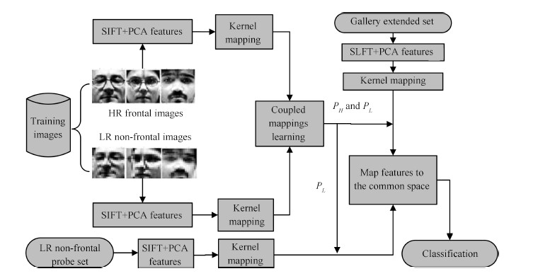
To overcome the limitations of the existing approaches,we propose a new method to handle poor resolution,pose and illumination variations jointly. The SIFT-based descriptors at fiducial locations on the face images are used as input features. This is because these descriptors are local features which are known to be robust to pose,illumination and scale variations [22] . During training,the features from HR frontal and LR non-frontal images are respectively mapped into two different high-dimensional feature spaces [24] by applying appropriate kernel functions. Then by using the enhanced discriminative analysis,we can learn two desired mappings from the kernel space to a common subspace where discrimination property is maximized. Finally,during testing,we use the extended gallery trick to solve the problem of a single gallery image per person and improve the recognition performance,and implement the classification step in the common space. Our method can achieve superior effectiveness and accuracy, which will be demonstrated in the experiments. The flowchart of the proposed approach with both training and testing stages is shown in Fig. 1.

|
Download:
|
| Fig. 1. The flowchart of the proposed approach. | |
The rest of this paper is organized as follows. Section Ⅱ describes the problem statement. Section Ⅲ presents coupled kernel-based enhanced discriminant analysis. In section Ⅳ,our gallery extended trick is introduced. Section Ⅴ demonstrates experiment results on the publicly available database. In Section Ⅵ,we conclude the paper. Detailed computation of the related terms can be seen in Appendix.
Ⅱ. PROBLEM STATEMENT A. Low-resolution Face RecognitionDifferent from conventional face recognition approaches,our proposed method needs to match LR non-frontal probe images with HR frontal gallery images. However,it is usually difficult to find a proper distance measure between a LR face image $l_{i}\in{\bf R}^{m}$ and a HR one $h_{j}\in{\bf R}^{M}$
\begin{align*} d_{ij}=D(l_{i},h_{j}). \end{align*}Obviously,since the dimensions of LR and HR features are not equal due to $m<M$,some common distances (e.g.,Euclidean distance) cannot be calculated directly. To solve the problem,the traditional two-step methods employ SR functions to project the LR image into the target HR space,and then calculate the distance in the HR space
\begin{align*} d_{ij}=D(f_{sr}(l_{i}),h_{j}), \end{align*}where $y=f_{sr}(l_{i})\in{\bf R}^{M}$ denotes the HR reconstructed image of the LR image $l_{i}$. Obviously,the first SR step is very important for the two-step methods. However,most existing SR methods aim to obtain a good visual reconstructed version,and they are usually not desired to improve the performance of the subsequent recognition step.
Different from previous methods,in [16],the data points in the original HR and LR feature spaces are projected into a common feature space by coupled mappings: one for LR feature vectors,$f_{L}:l_{i}\in{\bf R}^{m}\rightarrow {\bf R}^{d}$; the other for HR ones $f_{H}:h_{j}\in{\bf R}^{M}\rightarrow {\bf R}^{d}$. $ d $ represents the dimension of the common subspace. Then some distances can be computed in the common feature space by
$$D_{ij}=(f_{L}(l_{i}),f_{H}(h_{j})).$$Consequently,classification can be employed. Here,linear mapping functions are preferred. Specifically speaking,coupled mappings (CMs) $P_L$ and $ P_H$ with sizes of $m \times d$ and $M\times d$ are used to specify the mapping functions as $f_{L}(l_i) = P_{L}^{\rm T}l_i$ and $f_{H}(h_j) = P_{H}^{\rm T}h_{j}$,respectively.
B. Linear Discriminant AnalysisLDA [2] is a powerful classification method,in the sense that it can represent data and implement effective classification. Let $X=[x_{1},x_{2},\ldots,x_{N}]$ be a data set of given $M$-dimensional vectors of face images. Each data point belongs to one of $C$ object classes. LDA aims to find an optimal matrix $P$, which is determined by maximizing the between-class scatter while minimizing the within-class scatter of the training samples
\begin{align*} {\rm arg}\max\limits_{P} J(P)= \frac{P^{\rm T} S_b P}{P^{\rm T} S_{w}P}, \end{align*}where the between-class scatter matrix $S_{b}$ and the within-class scatter matrix $ S_{w}$ are defined as
\begin{align*} &S_{b}=\sum\limits_{i=1}^{C}(m_i-m)(m_i-m)^{\rm T},\\ &S_{w}=\sum\limits_{i=1}^{C}\sum\limits_{k=1}^{n_{i}}(x_k^i-m_i)(x_k^i-m_i)^{\rm T}, \end{align*}where $C$ is the total number of classes,$x_k^i$ is the $k$-th sample in class $i$,$m_i$ is the mean of samples in class $i$, $n_i$ is the number of samples in class $i$,$m$ is the total mean of all training samples.
By using the optimal matrix $P$,data are projected into a lower dimensional linear space where the features become more linearly separable.
Ⅲ. COUPLED KERNEL-BASED ENHANCED DISCRIMINANT ANALYSISOur aim is to match LR non-frontal probe images with HR frontal gallery ones. SIFT-based descriptors at all fiducial locations on the face images are taken as input features. During training,we use kernel functions to project the features from the HR frontal and LR non-frontal images into the two high-dimensional feature spaces. Then CKEDA learns two mappings from the two high-dimensional feature spaces to a common subspace where discrimination property is maximized by optimizing the objective function. In this section,we present how to learn the desired coupled mappings.
A. Related Formulation for CKEDALet the feature sets $H^{f}$ and $L^{p}$ respectively be corresponding to original HR frontal and LR non-frontal training images. Both of them can be expressed as $ H^{f}=[h_{1}^{f}, h_{2}^{f},\ldots,h_{N_t}^{f}]$ and $ L^{p}=[l_{1}^{p}, l_{2}^{p},\ldots, l_{N_t}^{p}]$,where $ N_{t}$ is the number of HR (or LR) training samples, $ h_{k}^{f} $ and $ l_{k}^{p} $ respectively denote the $k$-th HR and LR features.
First of all,the features $ h_{k}^{f} $ and $ l_{k}^{p} $ are respectively mapped onto two different high-dimensional feature spaces $V$ and $W$ by using kernel functions $\phi $ and $\varphi $.
| $ \begin{align} &\phi:{\bf R}^{M} \rightarrow V,\ h_{k}^{f}\mapsto\phi( h_{k}^{f}),\\ \end{align} $ | (1) |
| $ \begin{align} &\varphi:{\bf R}^{m} \rightarrow W,\ l_{k}^{p}\mapsto\varphi( l_{k}^{p}), \end{align} $ | (2) |
where ${\bf R}^M $ means the input feature space corresponding to HR training images,and ${\bf R}^m$ means the input feature space corresponding to LR training images. Two kernel feature sets are denoted as $\phi( H^{f})=[\phi( h_{1}^{f}),\phi( h_{2}^{f}),\ldots,\phi( h_{N_t}^{f})]$,and $\varphi( L^{p})=[\varphi(l^{p}_{1}),\varphi(l^{p}_{2}),\ldots,\varphi( l^{p}_{N_t})] $,respectively.
Then by using coupled mappings $ P_H $ and $ P_L$,the data from $\phi( H^{f})$ and $\varphi( L^{p})$ are simultaneously mapped into a common feature space ${\bf R}^d$ consisting of the data from two transformed feature sets $H^{f'}$ and $L^{p'}$. Here,$d $ is the dimension of the common feature space,$ H^{f'}=[h^{f'}_1, h^{f'}_2,\ldots,h^{f'}_{N_t}]$ and $L^{p'}=[l^{p'}_{1}, l^{p'}_{2},\ldots, l^{p'}_{N_t}]$. We can describe the corresponding data in this way:
| $ \begin{align} &[\phi( h_{1}^{f}),\phi( h_{2}^{f}),\ldots,\phi( h_{N_t}^{f})] \xrightarrow { P_{H}} [h^{f'}_1,h^{f'}_2,\ldots,h^{f'}_{N_t}],\\ \end{align} $ | (3) |
| $ \begin{align} &[\varphi( l^{p}_{1}),\varphi( l^{p}_{2}),\ldots,\varphi( l^{p}_{N_t})] \xrightarrow { P_{L}} [l^{p'}_{1}, l^{p'}_{2},\ldots,l^{p'}_{N_t}], \end{align} $ | (4) |
in which let projected features $ h_{k}^{f'} $ and $ l_{k}^{p'} $ be given by
| $ \begin{align} h_{k}^{f'}=P_{H}^{\rm T}\phi( h^{f}_k),\ \ \ l_k^{p'}= P_{L}^{\rm T} \varphi( l_{k}^{p}). \end{align} $ | (5) |
The mean of each class in the common space can be denoted as
| $ \begin{align} \mu_{i}'=\frac{1}{2N_i}\sum\limits_{k=1}^{N_i} \Big( h^{f'}_{i,k}+ l^{p'}_{i,k} \Big)=\frac{1}{2} P_H^{\rm T} \mu^{\phi}_{H_i}+\frac{1}{2}P_L^{\rm T}\mu^{\varphi}_{L_i} \end{align} $ | (6) |
where $ N_i $ means the number of the HR (or LR) samples in the $i$-th class,$h^{f'}_{i,k} $ and $ l^{p'}_{i,k} $ respectively denote the $k$-th projected features in the $k$-th class of $ H^{f'}$,$ L^{p'}$,$ \mu^{\phi}_{H_i} $ and $ \mu^{\varphi}_{L_i} $ respectively are the means of projected features in the $i$-th class of $ \phi( H^{f}) $ and $ \varphi(L^{p}) $.
The total mean of all projected features in the common space is defined as follows:
| $ \begin{align} \mu'=\frac{1}{2N_t}(\sum\limits_{k=1}^{N_t} h^{f'}_k+\sum\limits_{k=1}^{N_t} l^{p'}_k)= \frac{1}{2} P_H^{\rm T}\mu^{\phi}_{H}+\frac{1}{2} P_L^{\rm T}\mu^{\varphi}_{L}, \end{align} $ | (7) |
in which,$\mu^{\phi}_{H} $ and $\mu^{\varphi}_{L} $ represent respectively the means of the samples in $\phi( H^{f})$ and $\varphi(L^{p})$.
B. Our Objective FunctionMotivated by CMs and LDA,we hope to obtain two desired mappings $P_L$ and $ P_H$ from the kernel space to a common space where discrimination property is maximized. The proposed optimal objective function is very similar to the traditional LDA,which can be given by
| $ \begin{align} {\rm arg}\max\limits_{P} J( P_H,P_L)=\frac{ J_{b}(P_H,P_L)}{ J_{w}(P_H,P_L)}=\frac{P^{\rm T} S_b P}{P^{\rm T} S_{w}P}, \end{align} $ | (8) |
where the complete matrix of projections is given by $ P=\left[\begin{array}{c} P_H ;P_L \end{array} \right]$,$ J_{b}(P_H,P_L)=P^{\rm T} S_b P $ and $ J_{w}(P_H,P_L)=P^{\rm T} S_w P $,$ S_b $ and $ S_{w} $ respectively are expressed as the counterparts of the between-class scatter matrix and within-class scatter matrix in LDA.
Similarly,the term $ J_{w}(P_H,P_L)$ is used to minimize the distance between samples in the same class,while the term $ J_{b}(P_H,P_L)$ is used to maximize the distance between samples in different classes. Both of them play a similar role as of between-class scatter and the between-class scatter in LDA, respectively.
However,compared with traditional LDA,our $ J_{w}(P_H,P_L)$ and $ J_{b}(P_H,P_L)$ comprehensively integrate multiple discriminant factors,which could be formulated as
| $ \begin{align} &J_{w}(P_{H},P_{L})=w_{1} J_{w_1}+w_{2} J_{w_2}+w_{3} J_{w_3}+w_{4} J_{w_4},\\ \end{align} $ | (9) |
| $ \begin{align} &J_b(P_H,P_L)=b_{1} J_{b_1}+b_{2} J_{b_2}+b_{3} J_{b_3}+b_{4} J_{b_4}. \end{align} $ | (10) |
In (9),the weight control parameters $w_{1} ,w_{2},w_{3} , w_{4}$ are respectively corresponding to the four within-class distance minimizing terms $ J_{w_1},J_{w_2},J_{w_3} ,J_{w_4}$. The parameters $b_{1} ,b_{2},b_{3} ,b_{4} $ in (10) respectively denote weight control parameters of the four between-class distance maximizing terms $ J_{b_1},J_{b_2},J_{b_3},J_{b_4} $. The terms $J_{w_1}$ and $J_{b_1}$ could be obtained via applying the principle of traditional LDA while the other terms have different and novel meanings.
C. Improved Coupled Mappings LearningAll the four within-class distance minimizing terms are used to minimize the distance between samples in the same class while the four between-class distance maximizing terms are used to maximize the distance between the samples in different classes. However, each term has different effect on optimizing the objective function. Now we present the definitions of the related terms.
Based on the principle of traditional LDA,we can obtain the terms $J_{w_1}$ and $J_{b_1}$,which are denoted as
| $ \begin{align} & J_{w_1} = \frac{1}{2N_t}\sum\limits_{i=1}^{C} \sum\limits _{k=1} ^{N_i} \Big ( ( h^{f'}_{i,k}-\mu'_i)^2 + ( l^{p'}_{i,k}-\mu'_i)^2 \Big)\notag\\ &\qquad = P^{\rm T}S_{w_1}P,\\ \end{align} $ | (11) |
| $ \begin{align} &J_{b_1}= \frac{1}{2N_t}\sum\limits^{C}_{i=1}2N_i(\mu'_i-\mu')^2= P^{\rm T}S_{b_1}P, \end{align} $ | (12) |
here the detailed $S_{w_1}$ and $S_{b_1}$ are respectively presented in (A1) and (A2),$C$ is the number of all classes.
The aim of $J_{w_2} $ is to minimize the distance between each HR sample and the mean of LR samples both of which are in the same class,simultaneously,minimize the distance between each LR sample and the mean of HR samples both of which belong to the same class. Therefore,the second within-class distance minimizing term $J_{w_2} $ can be expressed as
| $ \begin{align} &J_{w_2}= \frac{1}{2N_t}\sum\limits_{i=1}^{C}\sum\limits_{k=1}^{N_i} \Big (( h_{i,k}^{f'}-\mu_{L_i}')^2 +(l_{i,k}^{p'}- \mu_{H_i}')^2 \Big )\notag\\ &\qquad = P^{\rm T} S_{w_2}P, \end{align} $ | (13) |
where $S_{w_2}$ is given by (A3),$ \mu_{L_i}' $ and $ \mu_{H_i}' $ respectively represent the means of the mapped feature vectors in c lass $i$ of $ H^{f'} $ and $ L^{p'}$.
Contrary to $J_{w_2} $,by substituting (13) into the following, we can obtain the term $J_{b_2}$,which is expressed as
| $ \begin{align} J_{b_2}=J_{2}-J_{w2} =P^{\rm T} S_{b_2}P, \end{align} $ | (14) |
where $ S_{b_2} = S_2- S_{w_2} $,$S_2$ is defined by (A4),and $J_{2} $ is given by
| $ \begin{align} & J_{2} = \frac{1}{2CN_t}\sum\limits_{i=1}^{C}\sum\limits_{k=1}^{N_t}\Big(( h_k^{f'}-\mu_{L_i}'^ {'})^2 +( l_k^{p'}- \mu_{H_i}')^2 \Big)\notag\\ &\qquad = P^{\rm T} S_{2}P, \end{align} $ | (15) |
where $J_{2} $ stands for the sum of the distance between each HR sample and the mean of LR samples in each class and that between each LR sample and the mean of HR samples in each class.
By using the term $ J_{w_3} $,we can minimize the distance between the mean of LR samples and the mean of HR samples both of which are in the same class. Thus the third within-class distance minimizing term $ J_{w_3} $ can be formulated as
| $ \begin{align} J_{w_3} =&\frac{1}{C} \sum\limits_{i=1}^{C}(\mu_{L_i}'-\mu_{H_i}')^{2}\notag\\ & = P^{\rm T} S_{w_3}P, \end{align} $ | (16) |
here $S_{w_3}$ can be computed by (A5).
Conversely,the term $J_{b_3}$ has the opposite effect. By substituting (16) into the following,$J_{b_3}$ can be obtained, which is denoted as
| $ \begin{align} J_{b_3}=J_{3}- J_{w3}=P^{\rm T}S_{b_3}P, \end{align} $ | (17) |
where $ S_{b_3} = S_3- S_{w_3} $,$S_3$ is defined by (A6),and $ J_{3}$ is denoted by
| $ \begin{align} J_{3}= \frac{1}{CC}\sum\limits_{j=1}^{C}\sum\limits_{i=1}^{C}( \mu_{L_i}'- \mu_{H_j}')^2 = P^{\rm T} S_{3}P, \end{align} $ | (18) |
$ J_{3}$ means the sum of the distance between the mean of LR samples in class $i $ and the mean of HR samples in class $ j $ in the common space.
By using the term $ J_{w_4}$,we could minimize the distance between each HR sample and each LR sample both of which belong to the same class in the common space. Accordingly,the fourth within-class distance minimizing term $ J_{w_4} $ can be given in this way
| $ \begin{align} J_{w4} = \frac{1}{N_tN_i}\sum\limits_{i=1}^{C} \sum\limits_{k=1}^{N_i}\sum\limits_{n=1}^{N_i} ( h_{i,k}^{f'}- l_{i,n}^{p'})^2 = P^{\rm T} S_{w_4}P, \end{align} $ | (19) |
in which,$S_{w_4}$ is expressed by (A7).
On the contrary,the term $J_{b_4}$ helps to maximize the distance between each HR sample in a certain class and each LR sample in another different class. By substituting (19) into the following,we can obtain $J_{b_4}$,which can be denoted by
| $ \begin{align} J_{b_4}=J_{4}-J_{w_4}=P^{\rm T} S_{b_4}P, \end{align} $ | (20) |
where $ S_{b_4} = S_4- S_{w_4} $,$S_4$ is given by (A8),and $J_{4} $ is expressed as
| $ \begin{align} J_{4}=\frac{1}{N_tN_t}\sum\limits_{k=1}^{N_t} \sum\limits_{n=1}^{N_t} ( h_k^{f'}- l_n^{p'})^2 = P^{\rm T} S_{4}P, \end{align} $ | (21) |
here $J_{4} $ denotes the sum of the distance between each HR sample and each LR sample in the common space.
By substituting (11),(13),(16) and (19) into (9),$ S_w $ in (8) can be given by
| $ \begin{align} S_w=w_1 S_{w_1}+w_2 S_{w_2}+w_3 S_{w_3}+w_4 S_{w_4}. \end{align} $ | (22) |
Similarly,by substituting (12),(14),(17) and (20) into (10),$ S_b $ in (8) can be written as follow:
| $ \begin{align} S_b=b_1 S_{b_1}+b_2S_{b_2}+b_3 S_{b_3}+b_4 S_{b_4}. \end{align} $ | (23) |
Let $Z=[\phi(H^f) \ 0;0 \ \varphi(L^p)]$,by using dual representation [19] ,the projections in $ P$ can be expressed as linear combinations of the feature $ Z $,i.e.,$P=ZU$. Therefore,the objective function (8) becomes
| $ \begin{align} J( U)=\frac{U^{\rm T}Z^{\rm T} S_b Z U}{U^{\rm T}Z^{\rm T} S_{w}ZU}=\frac{U^{\rm T} S_b^uU}{U^{\rm T}S_w^uU}, \end{align} $ | (24) |
where $S_b^u=Z^{\rm T} S_bZ$ and $S_w^u=Z^{\rm T} S_wZ $. The solution to the optimization function with respect to $U$ could be given by the first $ d $ largest generalized eigenvectors $ u $ of $ S_b^u u=\lambda S_w^u u $. In addition,since $ S_w^u $ is not always invertible,we need to perform a regularization operation, i.e.,$S_w^u+\zeta I$. $\zeta$ is a small positive value which is smaller than the smallest nonzero eigenvalue (e.g.,$\zeta=10^{-5}$).
Ⅳ. GALLERY EXTENDED TRICK FOR ONLY ONE GALLERY IMAGE PER PERSON PROBLEMThe proposed algorithm aims to solve the problem of the real-world face recognition systems. In addition to poor resolution, illumination and pose variation scenarios,real-world face recognition systems usually encounter only a single gallery image per person problem [25] . Actually,many existing face databases might only contain a limited number of gallery images such as a passport photo database. Most face recognition methods will suffer serious performance drop from one gallery image per person problem, and some of them even fail to work. To solve the problem,another significant contribution of this paper is to improve the recognition performance by using the proposed gallery extended trick.
We assume that the feature set $ G_h^{f} $ corresponding to HR frontal gallery images is the original gallery set,which is expressed by
| $ \begin{align} G_h^{f}=[g_h^1,g_h^{2},\ldots,g_h^{C_g}], \end{align} $ | (25) |
where $C_g $ is the number of all classes in $ G_h^{f} $. There is only one HR feature vector per subject in $ G_h^{f} $. Most existing LR face recognition approaches,for example [16, 17, 18, 19] , directly employ $ G_h^{f} $ as gallery set.
Different from the existing works,we consider to generate the LR gallery images by smoothing and down-sampling the HR gallery images corresponding to $ G_h^{f} $. And the LR frontal gallery images are of the same resolution as the LR training images. After extracting features from LR gallery images,the corresponding LR gallery set $G_l^{f} $ can be given by
| $ \begin{align} G_l^{f}=[g_l^1,g_l^{2},\ldots,g_l^{C_g}]. \end{align} $ | (26) |
Following the procedure in (1) and (2),we can obtain two kernel gallery sets,which could be expressed as $\phi( G^{f}_h)=[\phi( g_{h}^{1}),\phi( g_{h}^{2}),\ldots,\phi( g_{h}^{C_g})]$,and $\varphi( G^{f}_l)=[\varphi(g^{1}_{l}),\varphi(g^{2}_{l}), \ldots,\varphi( g^{C_g}_{l})] $,respectively.
By using the two mappings $P^{\rm T}_H$ and $P^{\rm T}_L$,the feature vectors in $\phi( G^{f}_h) $ and $ \varphi( G^{f}_l) $ are transformed into the common feature space ${\bf R}^d $ by
| $ \begin{align} g_h'^{i}= P^{\rm T}_H\phi(g_h^{i}),\ \ \ \ g_l'^{i}=P_L^{\rm T}\varphi(g_l^i), \end{align} $ | (27) |
where $\phi(g_h^{i})$ and $\varphi(g_l^i)$ denote the $i$-th feature vectors of $\phi( G^{f}_h)$ and $\varphi( G^{f}_l)$,respectively. So the two projected gallery sets could be written as $ G_h'=[ g_{h}'^{1},g_{h}'^{2},\ldots,g_{h}'^{C_g}]$ and $ G_l'=[ g_{l}'^{1},g_{l}'^{2},\ldots,g_{l}'^{C_g}]$.
We consider that the mean of feature vectors $ g_h'^{i} $ and $g_l'^{i}$ in class $i$ can be used as a new gallery feature in the common space
| $ \begin{align} g_m'^{i}=0.5( g_h'^{i}+g_l'^{i}). \end{align} $ | (28) |
Thus another added gallery set in the common feature space ${\bf R}^d $ can be formulated as $ G_m'=[g_{m}'^{1},g_{m}'^{2},\ldots,g_{m}'^{C_g}]$.
By synthesizing the feature vectors in $ G_h'$,$ G_l'$ and $G_m'$, the final gallery extension set $ G' $ in the common space can be given by
| $ \begin{align} G'=[G_h' ,G_l',G_m']. \end{align} $ | (29) |
According to (25) and (29),the feature vectors in $ G' $ are three times as many as the feature vectors in the original gallery set $ G_h^{f} $. Therefore,we believe this work would be a useful complement to the whole approach.
Ⅴ. EXPERIMENTSIn this section,extensive experiments aim to evaluate the performance of the proposed algorithm. To demonstrate the effectiveness of the proposed approach,we compare our algorithm with the state-of-the-art algorithm MDS [22] and two different SR techniques [26, 27] . The baseline algorithm is LR-HR,which matches directly the features from LR non-frontal probe images and HR frontal gallery ones.
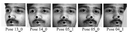
A. Datasets Used and Experimental SettingsAll the experiments are performed on the dataset from the Session 1 of multi-PIE [28] . The dataset contains images of 249 subjects. The images from 20 different illumination conditions with neutral expression,are in pose 04$\_$1,05$\_$0,13$\_$0 and 14$\_$0 (as shown in Fig. 2) in addition to frontal pose for gallery. The training set comprises of images of 100 randomly selected subjects. The rest subjects are used for testing. Therefore,there is no subject overlap between training and testing sets. The resolution of HR frontal gallery images is $60\,\times\,60 $,whereas the resolution of LR non-frontal probe images is kept at $20\,\times\,20 $. Unless otherwise stated,the same gallery and probe resolutions are used for the other experiments. The aligned face images are down-sampled from the HR to the LR by using bi-cubic interpolation technique.

|
Download:
|
| Fig. 2. Fiducial locations used for extracting SIFT descriptors for representing the input faces. | |
The SIFT descriptors computed at the fiducial locations (as shown in Fig. 2) are regarded as the input features. In Fig. 2,the hand-annotated fiducial points for Multi-PIE is given by Sharma [29] . Principal component analysis (PCA) [2] is used to reduce the dimensionality of the input features,and the first 100 PCA coefficients are needed. SIFT descriptors from the images of the HR frontal training set are used to generate PCA space.
For the algorithm MDS [22] used for comparison,the value of the parameter $\lambda $ is set to 0.9 and the output dimension $ m $ is set to 100,both of which are obtained by training; the kernel mapping $\phi(x)$ is fixed to $ x $ ,which is consistent with the corresponding setting in [22].
For our proposed method,the cubic kernel function is selected to achieve good classification performance; the output dimension $m $ is set to 80; all the weight control parameters are set as $w_{1}=1 ,w_{2}=0,w_{3}=1 ,w_{4}=1$ and $b_1=1;b_2=1,b_3=1,b_4=1 $.
B. Recognition Across Resolution,Pose,and IlluminationHere,two different modes for the experiments are performed to match HR frontal gallery images with LR probe ones in different poses and illuminations. In the two modes,there are different probe and gallery sets and classification techniques,which are set as follows.
For the first mode,just the 7th image per person constitutes gallery image set,images from all 20 illuminations of every person constitute probe image set, and Covariance [30] is employed to perform nearest neighbor classification. Table Ⅰ shows the rank-1 recognition accuracy of our approach compared to the approach MDS [22] . From Table Ⅰ,it is obvious that all the recognition results of our proposed algorithm across different poses are almost 20 % higher than MDS [22] ,which demonstrates the effectiveness of the proposed approach.
|
|
Table Ⅰ RANK-1 RECOGNITION RATE (%) OF OUR APPROACH COMPARED TO THE APPROACH [22] WITH THE FIRST MODE |
For the second mode,there is only one image per subject in the gallery and probe image sets,and images from one illumination form the gallery image set while images from another illumination form the probe image set. And the nearest neighbor classification is performed with Euclidean distance calculation [30] . The recorded recognition performance is the average rank-1 recognition accuracy averaged over all $C_{20}^2$ pairs of different illumination conditions forming gallery and probe sets. In this way,every two images are matched differently in resolution,pose and illumination condition. Note that the rest experiments conducted share the same gallery and probe sets and classification technique with the second mode.
Table Ⅱ represents the recognition results with the second mode. As is shown in Table Ⅱ, our proposed algorithm still considerably improves the recognition accuracy,compared to the algorithm MDS [22] . The outcome indicates that the proposed algorithm provides more pose robustness and discriminative information than MDS [22] .
|
|
Table Ⅱ RANK-1 RECOGNITION RATE (%) OF OUR APPROACH COMPARED TO THE APPROACH [22] WITH THE SECOND MODE |
From the results of the two experiments,the performance of the proposed algorithm across varying poses is much more excellent than MDS [22] . There are three reasons for the superior performance. Firstly,we utilize appropriate kernel function which can make data linearly separable. Secondly,the key of our approach is the enhanced discriminative analysis,which enables the projected features to be highly effective discriminant information in the common space. Thirdly,we improve the recognition accuracy by employing the gallery extended trick. Based on the three reasons,the proposed algorithm maintains excellent recognition performance in all the experiments. Therefore,it is believed that our algorithm is more robust to handle jointly poor resolution and pose variations than MDS [22] .
C. Recognition Performance Analysis with Super-resolution MethodsFor matching LR probe images with HR gallery images,the most common way is to first apply SR on LR probe images and then perform classification. Here,we use two different state-of-the-art SR techniques [26, 27] to obtain HR reconstructed images from the LR probe images. The result of comparisons with two SR methods on different subjects across different poses is shown in Table Ⅲ,where SR1 and SR2 respectively mean the SR technique [26] and the discriminative SR technique of [27]. It is evident that the proposed algorithm still performs better than MDS [22] . From Table Ⅲ,the two SR techniques show marked improvement upon the baseline algorithm LR-HR and the compared algorithm [26] ,while the performance of the proposed algorithm is not significantly improved. That is because the recognition accuracy of the proposed algorithm has been comparatively high,hence it is difficult to obtain further improvement.
|
|
Table Ⅲ RANK-1 RECOGNITION ACCURACY (%) WITH SR TECHNIQUES FOR FOUR DIFFERENT PROBE POSES |
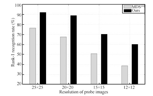
Now we evaluate the performance of our algorithm with varying resolutions of the probe images. The HR gallery images are maintained at a resolution $60\,\times\,60$ while the resolution of probe images are varied. We use four different probe resolutions $ 25\,\times\,25,20\,\times\,20, 15\,\times\,15$,and $12\,\times\,12$. LR probe images in pose 05$\_$0 are used for this experiment. The rank-1 recognition performance of our algorithm and MDS [22] is presented in Fig. 3. It is observed that the proposed algorithm performs notably well for wide range of low resolutions. It demonstrates that our algorithm is more robust for varying resolutions of the probe images than MDS [22] .

|
Download:
|
| Fig. 3. Rank-1 recognition rate for pose 05$\_$0 at four probe resolutions. | |
Pose has been a challenging and prominent problem in face recognition. And the pose problem is usually accompanied with poor resolution and illumination variations to jointly affect the performance of face recognition systems. To address the difficult problem,we propose a novel approach for matching HR gallery images in frontal pose with LR face images having considerable variations in pose and illumination. Our CKEDA aims to minimize the within-class distance while maximize the between-class distance in the common transformed space by using the learned coupled mappings. The data become linearly separable with the appropriate kernel functions. Moreover,the key of CKEDA is to apply the enhanced discriminative analysis. And by applying gallery extended trick,we solve the problem of a single gallery image per person and improve the recognition performance. All the experiment results demonstrate the superior performance for low-resolution face recognition with considerable variations in pose and illumination.
APPENDIXHere,we present the detailed calculation of the related terms associated with the proposed algorithms as follows.
1) $ J_{w_1} $
As shown in (11),the detailed formulation of the term $J_{w_1} $ is
| $ \begin{align*} J_{w_1} &= \frac{1}{2N_t}\sum\limits_{i=1}^{C} \sum\limits _{k=1} ^{N_i} \Big ( ( h^{f'}_{i,k}-\mu'_i)^2 + ( l^{p'}_{i,k}-\mu'_i)^2 \Big) \\ &=\left[P^{\rm T}_H \quad P^{\rm T}_L \right] \left[ \begin{array}{cc} W_{HH_1} & W_{HL_1}\\ W_{LH_1} & W_{LL_1} \end{array} \right] \left[\begin{array}{c} P_H \\ P_L \end{array} \right]\\ &= P^{\rm T} S_{w_1}P, \end{align*} $ | (A1) |
where $ S_{w_1}= [W_{HH_1} \ W_{HL_1}; W_{LH_1} \ W_{LL_1}] $,and the sub-matrices of matrix $ S_{w_1} $ are
\begin{align*} \begin{aligned} W_{HH_1}&=\frac{1}{2N_t}\sum\limits_{i=1}^{C} \Big( \sum\limits_{k=1}^{N_i} (\phi( h^{f}_{i,k})-\frac{1}{2}\mu_{H_i}^\phi) (\phi( h^{f}_{i,k})-\frac{1}{2}\mu_{H_i}^\phi)^{\rm T} \\ &\ \ \ \ +\frac{1}{4}N_i\mu_{H_i}^\phi(\mu_{H_i}^\phi)^{\rm T} \Big),\\ W_{HL_1}&=-\frac{1}{2N_t}\sum\limits_{i=1}^{C} \Big(\frac{1}{2}N_i\mu_{H_i}^\phi(\mu_{L_i}^\varphi)^{\rm T} \Big),\\ W_{LH_1}&= (W_{HL_1}) ^{\rm T} ,\\ W_{LL_1}&=\frac{1}{2N_t}\sum\limits_{i=1}^{C} \Big( \sum\limits_{k=1}^{N_i} (\varphi( l_{i,k}^p)-\frac{1}{2}\mu_{L_i}^\varphi) (\varphi(l_{i,k}^p)-\frac{1}{2}\mu_{L_i}^\varphi)^{\rm T} \\ &\ \ \ \ +\frac{1}{4}N_i\mu_{L_i}^\varphi(\mu_{L_i}^\varphi)^{\rm T} \Big). \end{aligned} \end{align*}2) $ J_{b_1} $
We can compute the term $J_{b_1} $ in (12) as follow:
| $ \begin{align*} J_{b_1} &= \frac{1}{2N_t}\sum\limits^{C}_{i=1}2N_i(\mu'_i-\mu')^2 \\ &=\left[P^{\rm T}_H \quad P^{\rm T}_L \right] \left[ \begin{array}{cc} B_{HH_1} & B_{HL_1}\\ B_{LH_1} & B_{LL_1} \end{array} \right] \left[\begin{array}{c} P_H \\ P_L \end{array} \right]\\ &= P^{\rm T} S_{b_1}P, \end{align*} $ | (A2) |
where $ S_{b_1} =[B_{HH_1} \ B_{HL_1};B_{LH_1} \ B_{LL_1}]$,and the sub-matrices of matrix $ S_{b_1} $ are denoted by
\begin{align*} B_{HH_1} &= \frac{1}{N_t} \sum \limits_{i=1}^{N_t} N_i (0.5\mu_{H_i}^{\phi}-0.5 \mu_{H}^{\phi}) (0.5\mu_{H_i}^{\phi}-0.5 \mu_{H}^{\phi})^{\rm T},\\ B_{HL_1} &=-\frac{1}{N_t} \sum \limits_{i=1}^{N_t} N_i (0.5\mu_{H_i}^{\phi}-0.5 \mu_{H}^{\phi}) (0.5\mu_{L_i}^{\varphi}-0.5 \mu_{L}^{\varphi}) ^{\rm T},\\ B_{LH_1} &=(B_{HL_1})^{\rm T},\\ B_{LL_1} &= \frac{1}{N_t} \sum \limits_{i=1}^{N_t} N_i (0.5\mu_{L_i}^{\varphi}-0.5 \mu_{L}^{\varphi}) (0.5\mu_{L_i}^{\varphi}-0.5 \mu_{L}^{\varphi}) ^{\rm T}. \end{align*}3) $ J_{w_2} $
From (13),the term $ J_{w_2} $ can be calculated as
| $ \begin{align*} J_{w_2} &= \frac{1}{2N_t}\sum\limits_{i=1}^{C} \sum\limits_{k=1}^{N_i} \Big (( h_{i,k}^{f'}- \mu_{L_i}^ {'})^2 +(l_{i,k}^{p'}- \mu_{H_i}^{'})^2 \Big ) \\&=\left[P^{\rm T}_H \quad P^{\rm T}_L \right] \left[\begin{array}{cc} W_{HH_2} & W_{HL_2} \\ W_{LH_2} & W_{LL_2} \end{array} \right] \left[\begin{array}{c} P_H \\ P_L \end{array} \right]\\ &= P^{\rm T} S_{w_2}P, \end{align*} $ | (A3) |
where $ S_{w_2}=[W_{HH_2} \ W_{HL_2};W_{LH_2} \ W_{LL_2}]$,and the blocks of matrix $ S_{w_2} $ are given by
\begin{align*} W_{HH_2}&=\frac{1}{2N_t}\sum\limits_{i=1}^{C} \Big( \sum\limits_{k=1}^{N_i}\phi( h^{f}_{i,k})\phi( h^{f}_{i,k})^{\rm T}+N_{i}\mu_{H_i}^\phi(\mu_{H_i}^\phi)^{\rm T} \Big ),\\ W_{HL_2} &=-\frac{1}{2N_t}\sum\limits_{i=1}^{C} \sum \limits_{k=1}^{N_i} \Big( \phi( h^{f}_{i,k}) ( \mu_{L_i}^\varphi)^{\rm T} + \mu_{H_i}^\phi \varphi( l_{i,k}^p)^{\rm T} \Big),\\ W_{LH_2} & =(W_{HL_2})^{\rm T},\\ W_{LL_2} &=\frac{1}{2N_t}\sum\limits_{i=1}^{C} \Big( \sum \limits_{k=1}^{N_i} \varphi( l^{p}_{i,k})\varphi(l^{p}_{i,k})^{\rm T}+N_{i}\mu_{L_i}^\varphi(\mu_{L_i}^\varphi)^{\rm T} \Big). \end{align*}4) $ J_{2} $
As shown in (15),the term $J_{2} $ can be computed as
| $ \begin{align*} J_2 &= \frac{1}{2CN_t}\sum\limits_{i=1}^{C}\sum\limits_{k=1}^{N_t}\Big(( h_k^{f'}-\mu'_{Li})^2 +( l_k^{p'}- \mu'_{Hi})^2 \Big) \\ &=\left[P^{\rm T}_H \quad P^{\rm T}_L \right] \left[ \begin{array}{cc} T_{HH_2} & T_{HL_2}\\ T_{LH_2} & T_{LL_2} \end{array} \right] \left[\begin{array}{c} P_H \\ P_L \end{array} \right]\\ &= P^{\rm T} S_{2}P, \end{align*} $ | (A4) |
where $S_{2}=[T_{HH_2} \ T_{HL_2}; T_{LH_2}\ T_{LL_2}]$,the sub-matrices of matrix $ S_{2}$ are expressed as
\begin{align*} T_{HH_2} &= \frac{1}{2CN_t}\sum\limits_{i=1}^{C}\sum\limits_{k=1}^{N_t} \Big( \phi({ h^{f}_k})\phi({ h^{f}_k})^{\rm T}+{\mu_{H_i}^\phi}({\mu_{H_i}^\phi})^{\rm T} \Big),\\ T_{HL_2} &=-\frac{1}{2CN_t}\sum\limits_{i=1}^{C}\sum\limits_{k=1}^{N_t} \Big ( \phi({ h^{f}_k}) ( \mu_{L_i}^{\varphi})^{\rm T}+\mu_{H_i}^{\phi} \varphi({ l_k^p})^{\rm T}\Big),\\ T_{LH_2} &=({T_{HL_2}})^{\rm T},\\ T_{LL_2} &= \frac{1}{2CN_t}\sum\limits_{i=1}^{C}\sum\limits_{k=1}^{N_t} \Big ( \varphi({l^{p}_k})\varphi({ l^{p}_k})^{\rm T}+{\mu_{L_i}^\varphi}({\mu_{L_i}^\varphi})^{\rm T}\Big ). \end{align*}5) $ J_{w_3} $
From (16),the term $J_{w_3} $ can be expressed as
| $ \begin{align*} J_{w_3} &= \frac{1}{C} \sum\limits_{i=1}^{C}(\mu'_{L_i}-\mu'_{H_i})^{2} \\ &=\left[P^{\rm T}_H \quad P^{\rm T}_L \right] \left[ \begin{array}{cc} W_{HH_3} & W_{HL_3}\\ W_{LH_3} & W_{LL_3} \end{array} \right] \left[\begin{array}{c} P_H \\ P_L \end{array} \right]\\ &= P^{\rm T} S_{w_3}P, \end{align*} $ | (A5) |
where $ S_{w_3} =[W_{HH_3} \ W_{HL_3};W_{LH_3} \ W_{LL_3}]$,and the sub-matrices of matrix $ S_{w_3} $ are formulated as
\begin{align*} W_{HH_3} &= \frac{1}{C} \sum \limits_{i=1}^{C}\mu_{H_i}^{\phi}(\mu_{H_i}^{\phi})^{\rm T}, \\ W_{HL_3} &=-\frac{1}{C} \sum \limits_{i=1}^{C}\mu_{H_i}^{\phi}( \mu_{L_i}^{\varphi})^{\rm T}, \\ W_{LH_3}&=({W_{HL_3}})^{\rm T}, \\ W_{LL_3} &= \frac{1}{C} \sum \limits_{i=1}^{C}\mu_{L_i}^\varphi(\mu_{L_i}^\varphi)^{\rm T}. \end{align*}6) $ J_3$
As shown in (18),we can calculate the term $J_{3}$ as
| $ \begin{align*} J_3 &= \frac{1}{CC}\sum\limits_{j=1}^{C}\sum\limits_{i=1}^{C} ( \mu'_{Li}- \mu'_{Hj})^2 \\ &=\left[P^{\rm T}_H \quad P^{\rm T}_L \right] \left[ \begin{array}{cc} T_{HH_3} & T_{HL_3}\\ T_{LH_3} & T_{LL_3} \end{array} \right] \left[\begin{array}{c} P_H \\ P_L \end{array} \right]\\ &= P^{\rm T}S_{3}P, \end{align*} $ | (A6) |
where $ S_{b_3}=[T_{HH_3} \ T_{HL_3}; T_{LH_3} \ T_{LL_3}] $,the sub-matrices of matrix $S_{b_3} $ are
\begin{align*} T_{HH_3} &= \frac{1}{CC}\sum\limits_{j=1}^{C}\sum\limits_{i=1}^{C} {\mu_{H_i}^\phi}({\mu_{H_i}^\phi})^{\rm T},\\ T_{HL_3} &=- \frac{1}{CC}\sum\limits_{j=1}^{C}\sum\limits_{i=1}^{C} \mu_{H_i}^{\phi}( \mu_{L_j}^{\varphi})^{\rm T},\\ T_{LH_3} &=({T_{HL_3}})^{\rm T},\\ T_{LL_3} &= \frac{1}{CC}\sum\limits_{j=1}^{C}\sum\limits_{i=1}^{C} \mu_{L_j}^{\varphi}(\mu_{L_j}^{\varphi})^{\rm T}. \end{align*}7) $ J_{w_4} $
From (19),the term $ J_{w_4} $ can be computed as
| $ \begin{align*} J_{w4} &= \frac{1}{N_tN_i}\sum\limits_{i=1}^{C} \sum\limits_{k=1}^{N_i}\sum\limits_{n=1}^{N_i} ( h_{i,k}^{f'}- l_{i,n}^{p'})^2 \\ &=\left[P^{\rm T}_H \quad P^{\rm T}_L \right] \left[ \begin{array}{cc} W_{HH_4} & W_{HL_4}\\ W_{LH_4} & W_{LL_4} \end{array} \right] \left[\begin{array}{c} P_H \\ P_L \end{array} \right]\\ &= P^{\rm T}S_{w_4}, \end{align*} $ | (A7) |
where $S_{w_4} =[W_{HH_4} \ W_{HL_4}; W_{LH_4} \ W_{LL_4}] $,and the sub-matrices of matrix $ S_{w_4} $ are denoted by
\begin{align*} W_{HH_4}&=\frac{1}{N_tN_i}\sum\limits_{i=1}^{C} \sum\limits_{k=1}^{N_i} \sum\limits_{n=1}^{N_i}\phi( h^{f}_{i,k})\phi(h^{f}_{i,k})^{\rm T},\\ W_{HL_4}&=-\frac{1}{N_tN_i}\sum\limits_{i=1}^{C} \sum\limits_{k=1}^{N_i} \sum\limits_{n=1}^{N_i}\phi(h^{f}_{i,k})\varphi(l^{p}_{i,k})^{\rm T},\\ W_{LH_4} &=(W_{HL_4})^{\rm T},\\ W_{LL_4} &=\frac{1}{N_tN_i}\sum\limits_{i=1}^{C} \sum\limits_{k=1}^{N_i} \sum\limits_{n=1}^{N_i}\varphi( l^{p}_{i,k})\phi( l^{p}_{i,k})^{\rm T}. \end{align*}8) $ J_4$
As shown in (21),the term $ J_4$ is computed in the way
| $ \begin{align*} J_4 &= \frac{1}{N_tN_t}\sum\limits_{k=1}^{N_t} \sum\limits_{n=1}^{N_t} ( h_k^{f'}-l_n^{p'})^2 \\ &=\left[P^{\rm T}_H \quad P^{\rm T}_L \right] \left[ \begin{array}{cc} T_{HH_4} & T_{HL_4}\\ T_{LH_4} & T_{LL_4} \end{array} \right] \left[\begin{array}{c} P_H \\ P_L \end{array} \right]\\ &= P^{\rm T} S_{4}P, \end{align*} $ | (A8) |
where $ S_{4} =[T_{HH_4} \ T_{HL_4};T_{LH_4} \ T_{LL_4}] $,and the sub-matrices of matrix $S_{4}$ are
\begin{align*} T_{HH_4}&= \frac{1}{N_tN_t}\sum\limits_{k=1}^{N_t} \sum\limits_{n=1}^{N_t} \phi({ h^{f}_k})\phi({ h^{f}_k})^{\rm T},\\ T_{HL_4}&=- \frac{1}{N_tN_t}\sum\limits_{k=1}^{N_t} \sum\limits_{n=1}^{N_t} \phi({ h^{f}_k})\varphi({ l^{p}_n})^{\rm T},\\ T_{LH_4} &=(T_{HL_4})^{\rm T},\\ T_{LL_4} &= \frac{1}{N_tN_t}\sum\limits_{k=1}^{N_t} \sum\limits_{n=1}^{N_t} \varphi({ l^{p}_n})\varphi({l^{p}_n})^{\rm T}. \end{align*}| [1] | Bartlett M S, Movellan G R, Sejnowski T J. Face recognition by independent component analysis. IEEE Transactions on Neural Networks,2002, 13(6): 1450-1464 |
| [2] | Belhumeur P N, Hespanha J P, Kriegman D. Eigenfaces vs. Fisherfaces: recognition using class specific linear projection. IEEE Transactions on Pattern Analysis and Machine Intelligence, 1997, 19(7): 711-720 |
| [3] | Gao Y S, Leung M K H. Face recognition using line edge map. IEEE Transactions on Pattern Analysis and Machine Intelligence, 2002, 24(6): 764-779 |
| [4] | He X F, Yan S C, Hu Y X, Niyogi P. Face recognition using Laplacianfaces. IEEE Transactions on Pattern Analysis and Machine Intelligence, 2005, 27(3): 328-340 |
| [5] | Hennings-Yeomans P H, Baker S, Kumar V K V. Simultaneous superresolution and feature extraction for recognition of low resolution faces. In: Proceedings of the 2008 IEEE Conference on Computer Vision and Pattern Recognition. Anchorage, AK: IEEE, 2008. 1-8 |
| [6] | Blanz V, Vetter T. Face recognition based on fitting a 3D morphable model. IEEE Transactions on Pattern Analysis and Machine Intelligence, 2003, 25(9): 1063-1074 |
| [7] | Zhang L, Samaras D. Face recognition from a single training image under arbitrary unknown lighting using spherical harmonics. IEEE Transactions on Pattern Analysis and Machine Intelligence, 2006, 28(3): 351-363 |
| [8] | Prince S J D, Warrell J, Elder J H, Felisberti F M. Tied factor analysis for face recognition across large pose differences. IEEE Transactions on Pattern Analysis and Machine Intelligence, 2008, 30(6): 970-984 |
| [9] | Baker S, Kanade T. Hallucinating faces. In: Proceedings of the 4th IEEE International Conference on Automatic Face and Gesture Recognition. Grenoble: IEEE, 2000. 83-88 |
| [10] | Hennings-Yeomans P H, Kumar V K V , Baker S. Robust low-resolution face identification and verification using high-resolution features. In: Proceedings of the 16th IEEE International Conference on Image Processing. Cairo: IEEE, 2009. 33-36 |
| [11] | Chakrabarti A, Rajagopalan A, Chellappa R. Super-resolution of face images using kernel PCA-based prior. IEEE Transactions on Multimedia, 2007, 9(4): 888-892 |
| [12] | Liu C, Shum H Y, Freeman W T. Face hallucination: theory and practice. International Journal of Computer Vision, 2007, 75(1): 115-134 |
| [13] | Marciniak T, Dabrowski A, Chmielewska A, Weychan R. Face recognition from low resolution images. In: Proceedings of the 5th International Conference on Multimedia Communications, Services, and Security. Krakow, Poland: Springer, 2012. 220-229 |
| [14] | Hwang W, Huang X, Noh K, Kim J. Face recognition system using extended curvature gabor classifier bunch for low-resolution face image. In: Proceedings of the 2011 IEEE Conference on Computer Vision and Pattern Recognition Workshops. Colorado Springs, CO: IEEE, 2011. 15-22 |
| [15] | Phillips P J, Flynn P J, Scruggs T, Bowyer K W, Chang J, Hoffman K, Marques J, Min J, Worek W J. Overview of the face recognition grand challenge. In: Proceedings of the 2005 IEEE Conference on Computer Vision and Pattern Recognition. San Diego, CA, USA: IEEE, 2005. 947-954 |
| [16] | Li B, Chang H, Shan S G, Chen X L. Low-resolution face recognition via coupled locality preserving mappings. IEEE Signal Processing Letters, 2010, 17(1): 20-23 |
| [17] | He X F, Yan S C, Hu Y X, Niyogi P, Zhang H J. Face recognition using Laplacian faces. IEEE Transactions on Pattern Analysis and Machine Intelligence, 2006, 27(3): 328-340 |
| [18] | Zhou C T, Zhang Z W, Yi D, Lei Z, Li S Z. Low-resolution face recognition via simultaneous discriminant analysis. In: Proceedings of the 2011 International Joint Conference on Biometrics (IJCB11). Washington, DC, USA: IEEE, 2011. 1-6 |
| [19] | Ren C X, Dai D Q, Yan H. Coupled kernel embedding for low-resolution face image recognition. IEEE Transactions on Image Processing, 2013, 21(8): 3770-3783 |
| [20] | Ren C X, Dai D Q. Piecewise regularized canonical correlation discrimination for low resolution face recognition. In: Proceedings of the 2010 Chinese Conference on Pattern Recognition. Chongqing, China: IEEE, 2010. 1-5 |
| [21] | Biswas S, Bowyer K W, Flynn P J. Multidimensional scaling for matching low-resolution face images. IEEE Transactions on Pattern Analysis and Machine Intelligence, 2012, 34(10): 2019-2030 |
| [22] | Biswas S, Aggarwal G, Flynn P J, Bowyer K W. Pose-robust recognition of low-resolution face images. IEEE Transactions on Pattern Analysis and Machine Intelligence, 2013, 35(12): 3037-3049 |
| [23] | Lowe D G. Distinctive image features from scale-invariant keypoints. International Journal of Computer Vision, 2004, 60(2): 91-110 |
| [24] | Schöolkopf B, Smola A, Möuller K. Nonlinear component analysis as a kernel eigenvalue problem. Neural Computation, 1998, 10(5): 1299-1319 |
| [25] | Tan X Y, Chen S C, Zhou Z H, Zhang F Y. Face recognition from a single image per person: a survey. Pattern Recognition, 2012, 39(9): 1725-1745 |
| [26] | Kim I K, Kwon Y. Single-image super-resolution using sparse regression and natural image prior. IEEE Transactions on Pattern Analysis and Machine Intelligence, 2010, 32(6): 1127-1133 |
| [27] | Zou W W W, Yuen P C. Very low resolution face recognition problem. IEEE Transactions on Image Processing, 2012, 21(1): 327-340 |
| [28] | Gross R, Matthews I, Cohn J, Kanade T, Baker S. Multi-PIE. In: Proceedings of the 8th IEEE International Conference on Automatic Face & Gesture Recognition. Amsterdam: IEEE, 2008. 1-8 |
| [29] | Sharma A, Haj M A, Choi J, Davis L S, Jacobs D W. Robust pose invariant face recognition using coupled latent space discriminant analysis. Computer Vision and Image Understanding, 2012, 116(11): 1095-1110 |
| [30] | Verma T, Sahu R K. PCA-LDA based face recognition system & results comparison by various classification techniques. In: Proceedings of the 2013 IEEE International Conference on Green High Performance Computing. Nagercoil: IEEE, 2008. 1-7 |