 2016, Vol.3


Continuous-time (CT) system identification plays an important role in many application problems because most dynamical systems encountered in the physical world are CT in nature[1, 2, 3, 4]. In general,the approaches for CT system identification can be classified into two categories: the indirect approach and the direct approach. The indirect approach uses discretization and discrete-time (DT) identification methods to obtain DT model first and then converts it to CT form,while the direct approach identifies the CT model directly from the input and output measurement data. Although the indirect approach has dominated the CT system identification for some time with benefits of well-performing DT system identification methods developed over last decades,there are still difficulties in this approach due to primarily the estimation of equivalent DT model and the conversion of equivalent DT model to its CT counterpart. Difficulties,such as nonminimum phase and undesirable sensitivity problems,are encountered when the sampling time interval is either too small or too large[2],which makes the indirect approach difficult to implement in some practical applications.
The direct approach can overcome the difficulties associated with the indirect approach,but it needs to compute the time-derivatives of input/output (I/O) variables,which is a nontrivial and delicate task in the presence of measurement noise[2, 3, 5]. Many methods have been devised to circumvent the difficulty in reconstructing the time-derivatives,and a concise survey can be found in [2]. The generalized Poisson moment functional (GPMF)[1, 6, 7] is one of the efficient methods to circumvent the difficulty of time-derivative and improve the accuracy of CT identification. GPMF belongs to the category of linear filtering method which reconstructs the time derivative of I/O data with Poisson moment function. Its digital implementation and parameter setup are detailed in [1]. GPMF has been extensively applied to system identification,industrial control and micro-electronics areas[1, 8, 9].
As a convex heuristic of the rank minimization problem,nuclear norm minimization (NNM) has recently been extensively studied[10, 11, 12, 13, 14]. NNM is guaranteed to find the minimum rank matrix under suitable assumptions and can be solved by the iterative reweighted algorithms[15] or the interior point method[10]. Due to the convex relaxation of rank minimization[13, 16],NNM has been used in SIM to minimize the rank of Hankel matrix and determine the order of the model[10, 12, 17, 18, 19, 20]. As we all know,subspace identification method (SIM)[21],is an effective and easy-to-implement identification method for linear time-invariant (LTI) system. In theory,the system order is equal to the rank of Hankel matrix which,in turn,equals the number of nonzero singular values of the matrix. However,the I/O variables in practice often contain noise that perturbs the singular values of Hankel matrix and makes the order determination of SIM unreliable.
The NNM can overcome the difficulty of model order determination in SIM and obtain a correct order identification when the priori order is unknown. However,by now the results of NNM based subspace system identification are confined to the DT models and do not carry over easily to CT case,due to the difference between the DT and CT Hankel matrices. Furthermore,the time-derivative in continuous-time SIM (CSIM) can bring in extra errors due to the measurement noise in the I/O data. How to correctly identify the CT system where the model order is not known a priori is still a big challenge in system identification field.
In light of the above observations,this paper proposes a novel method that incorporates NNM into the GPMF-based subspace method for the CT system identification. The proposed method not only circumvents the difficulty in the computation of time-derivatives of the noise corrupted I/O variables,but also alleviates the difficulty of model order estimation in the CT subspace identification. The algorithm for solving the NNM in CT SIM is deduced by ADMM and NNM is extended to CT cases for the first time.
The paper is organized as follows. Section Ⅱ reviews the basic DT SIM and its NNM. Section Ⅲ introduces the theory and algorithm of the GPMF method. Section Ⅳ analyzes the NNM and presents the framework of the novel hybrid algorithm. In Section Ⅴ,two typical numerical examples are presented to evaluate the GPMF based subspace identification with NNM,and concluding remarks are given in Section Ⅵ.
The notations used in the paper are standard. The estimate of a variable $x$ is denoted by $\hat{x}$. For a matrix $X$,$\|X\|_F$ denotes its Frobenius norm,$\|X\|_*$ its nuclear norm and $X^{\bot}$ its orthogonal projection. $s$ represents the Laplace variable. $R$ denotes the set of all real numbers,${\bf R}^+$ the set of all positive real numbers,and $R^{+*}$ the projectively extended positive real numbers. $I_q \in {\bf R}^{q\times q}$ is the identity matrix and $0_q \in {\bf R}^{q\times q}$ is the null matrix where all elements are zeros.
Ⅱ. DISCRETE-TIME SUBSPACE IDENTIFICATION AND NUCLEAR NORM MINIMIZATION A. Discrete-time Subspace IdentificationConsider a linear time-invariant DT state space system[22]:
| \begin{array}{l} x(k+1)=A x(k) + B u(k), \end{array} | (1) |
| \begin{array}{l} y(k) = C x(k) + D u(k), \end{array} | (2) |
where $u(k) \in R^m$ and $y(k) \in R^p$ are respectively the input and output,$x(k) \in R^n$ is the state vector,and $A \in R^{n\times n}$,$B \in {\bf R}^{n\times m}$,$C \in R^{p\times n}$,$D \in {\bf R}^{p\times m}$ are the state,input,output and feed-forward matrices,respectively.
It is well known that for the conventional discrete-time SIM (DSIM)[22],the basic state space model shown in (1) and (2) can be rewritten in matrix form at the periodic instants $k = 0, 1,...,N-1$,where $N$ is the number of samples.
| \begin{array}{l} Y_{0|r-1} = \mathcal{O}_r X_0 +\varPsi_r U_{0|r-1}. \end{array} | (3) |
In (3)
| \begin{array}{l} {Y_{0|r - 1}} = \left[ {\begin{array}{*{20}{c}} {y(0)}&{y(1)}& \cdots &{y(N - r)}\\ {y(1)}&{y(2)}& \cdots &{y(N - r + 1)}\\ \vdots & \vdots & \ddots & \vdots \\ {y(r - 1)}&{y(r)}& \cdots &{y(N - 1)} \end{array}} \right]\\ \;\;\;\;\;\;\;\;\; \in {R^{rp \times (N - r + 1)}}, \end{array} | (4) |
$U_{0|r-1}$is the same as $Y_{0|r-1}$ except its elements are the input variable $u(k)$,$k = 0,1,...,N-1$,and $X_0=[x(0) x(1) \cdots x(N-r)] \in R^{n \times (N-r+1)}$. Both $Y_{0|r-1}$ and $U_{0|r-1}$ are the standard block Hankel matrices with the identical structure for the DSIM. $\mathcal{O}_r \in {\bf R}^{rp\times n}$ is the observability matrix and $\varPsi_r \in {\bf R}^{rp \times rm}$ is the system matrix of (1) and (2) with the structures shown in (13) and (14).
However,SIM may suffer from incorrect estimation of the model order. Theoretically,when $r$ and $N$ approach to infinity,the model order is given by[22]
| \begin{array}{l} n={\rm rank}(Y_{0|r-1} U_{0|r-1}^{\bot}), \end{array} | (5) |
where $U_{0|r-1}^{\bot}$ is the projection of $U_{0|r-1}$,whose columns span the nullspace of $U_{0|r-1}$ . The model order is normally determined by the number of singular values of $Y_{0|r-1} U_{0|r-1}^{\bot}$ that are above the median value of the singular values in a logarithmic scale[17]. However,this approach can be difficult in practice as the singular values may become inseparable when the I/O measurements are noise corrupted. Some examples of bad cases are presented by Fazel et al.[12] to show this problem.
B. Nuclear Norm Minimization for Discrete-time Subspace IdentificationThe NNM of a matrix $X$ is the heuristic convex relaxation of the rank minimization of X[16]. When NNM is applied to the DSIM, it is usually used to constraint the rank of matrix product $Y_{0|r-1} U_{0|r-1}^{\bot}$ which determines the model order. Denote $\|X\|_*=\sum_{i=1}^{{\rm min}\{m,n\}}\sigma_i(X)$ as the nuclear norm of $X \in R^{m\times n}$ where $\sigma_i(X)$ is the $i\text{th}$ singular value of the matrix $X$.
Based on results of [12] ,the DT subspace identification can be cast into the following optimization problem
| \begin{array}{l} \begin{aligned} &\min_{y_d} ~~ \|Y_{0|r-1}(y_d) U_{0|r-1}^{\bot}\|_* ,\\ &{\rm s.t.} ~~~~\|y_d-\tilde{y}_d\| \leq \varepsilon. \end{aligned} \end{array} | (6) |
In (6)
| \begin{array}{l} \tilde{y}_d := [\tilde{y}(0)~ \tilde{y}(1)~ \cdots~ \tilde{y}(N-1)] \in R^{p\times N}, \end{array} | (7) |
where $\tilde{y}(\cdot)$ is the measured system output containing noise,$y_d \in R^{p\times N}$ is the optimization variable defined similarly as $\tilde{y}_d$ but with $\tilde{y}(\cdot)$ replaced by the computed system output obtained from the optimization process,$y_d-\tilde{y}_d$ is the output error,and $Y_{0|r-1}(y_d)$ is similar to $Y_{0|r-1}$ given in (4) with the elements from $y_d$ .
Extensive analysis and simulation results in [12] have shown that the minimization of $\|Y_{0|r-1}(y_d) U_{0|r-1}^{\bot}\|_*$ dramatically improves the performance of SIM,especially in the estimation of model order. However,it is not straightforward to extend the above NNM based DSIM to the CT case,because of the time-derivative of I/O data and the different structures of Hankel matrix in the CT subspace identification. The different structures of Hankel matrix make the solution of NNM in DT case cannot be directly used to solve NNM in CT case.
Ⅲ. Continuous-Time Subspace Identification with GPMF A. Continuous-time Subspace IdentificationConsider a linear time-invariant CT state space system
| \begin{array}{l} \dot{x}(t)=Ax(t)+Bu(t), \end{array} | (8) |
| \begin{array}{l} y(t)=Cx(t)+Du(t), \end{array} | (9) |
where $u(t)\in R^m$ and $y(t)\in R^p$ are respectively the input and output,$x(t)\in R^n$ is the state vector,and $A\in R^{n\times n}$,$B\in R^{n\times m}$,$C\in {\bf R}^{p\times n}$,$D\in R^{p\times m}$ are the state,input, output and feed-forward matrices,respectively. Taking the time-derivative on (9) and substituting $\dot{x}(t)$ into (8),then repeating the time-derivative of $y(t)$ up to the $(r-1)$-{th} order,the state space representation (8) and (9) can be converted to the matrix form[2]
| \begin{array}{l} Y_{0|r-1}^C = \mathcal{O}_r^C X_0^C +\varPsi_r^C U_{0|r-1}^C. \end{array} | (10) |
Equation (10) is the basis for the CSIM where
| \begin{array}{l} Y_{0|r - 1}^C = \left[ {\begin{array}{*{20}{c}} {y({t_1})}&{y({t_2})}& \cdots &{y({t_N})}\\ {\dot y({t_1})}&{\dot y({t_2})}& \cdots &{\dot y({t_N})}\\ \vdots & \vdots & \ddots & \vdots \\ {{y^{(r - 1)}}({t_1})}&{{y^{(r - 1)}}({t_2})}& \cdots &{{y^{(r - 1)}}({t_N})} \end{array}} \right]\\ \;\;\;\;\;\;\;\;\;\; \in {R^{pr \times N}}, \end{array} | (11) |
| \begin{array}{l} X_0^C=[x(t_1)~ x(t_2)~ \cdots~ x(t_N)]\in R^{n\times N}, \end{array} | (12) |
where $(\cdot)^{(r-1)}:=\frac{{\rm d}^{r-1}(\cdot)}{{\rm d}t^{r-1}}$ and $U_{0|r-1}^C$ is identical to $Y_{0|r-1}^C$ in structure but with $y(t)$ replaced by $u(t)$,
| \begin{array}{l} \mathcal{O}_r^C=\left[C^{\rm T}~ (CA)^{\rm T}~ \cdots ~(CA^{r-1})^{\rm T}\right]^{\rm T} \in R^{pr\times n}, \end{array} | (13) |
and
| \begin{array}{l} \Psi _r^C = \left[ {\begin{array}{*{20}{c}} D&0& \cdots &{}\\ {CB}& \ddots & \ddots &{}\\ \vdots &{}& \ddots & \ddots \\ \vdots &{}& \ddots & \ddots \\ {C{A^{r - 2}}B}&{C{A^{r - 3}}B}& \cdots &{CB} \end{array}\begin{array}{*{20}{c}} 0\\ \vdots \\ {}\\ 0\\ D \end{array}} \right]\\ \;\;\;\;\;\;\;\; \in {R^{pr \times mr}}. \end{array} | (14) |
The time sequence $t=\{t_1,t_2,...,t_N\}$ is used to represent different sampling instants,which are not necessarily equidistant. $\mathcal{O}_r^C (r>n)$ is the observability matrix and $\varPsi_r^C$ is the (block Toeplitz) system matrix of (8) and (9). Although the matrices $Y_{0|r-1}^C$ and $U_{0|r-1}^C$ do not have the structure of standard Hankel matrix,they will still be called Hankel matrix hereafter for simplification of terminology and convenience of comparison with the DSIM.
Note that (10) is in the same form as its DT counterpart (3), hence the computation procedures of the DSIM can be readily used here to obtain the CT state-space model for the system (8) and (9). In particular,when $r$ and $N$ are sufficiently large,the model order $ n={\rm rank}(Y_{0|r-1}^C U_{0|r-1}^{C\bot})$ can be determined by calculating the nonzero singular values of $(Y_{0|r-1}^C U_{0|r-1}^{C\bot})$[20],where $U_{0|r-1}^{C\bot}$ is the projection of $U_{0|r-1}^{C}$. These computations are based on $(Y_{0|r-1}^C U_{0|r-1}^{C\bot})$ which consists of the time-derivatives of the system output and input variables up to the order $r-1$. Since the measured system output is always noise corrupted,its direct differentiations,especially the high order ones,will greatly amplify the noise and hence distort the identification results. To overcome this problem,the generalized Poisson moment functional filtering is often used in the CT subspace identification to obtain the derivatives of system input and output variables.
B. Generalized Poisson Moment Functional (GPMF) FilteringThe $j$-th order GPMF transformation of a scalar signal over $[0,t]$ is given by the following convolution product[23]
| \begin{array}{l} M_j\{h(t)\}:=\int_0^t g_j(\tau) h(t-\tau) {\rm d}\tau = [g_j*h](t), \end{array} | (15) |
where $g_j(t)=\beta^{j+1} \frac{t^j}{j!} {\rm e}^{-\lambda t} $ is the $j$-th Poisson pulse function,$\lambda \in R^+$ and $\beta \in R^{+*}$ are the Poisson filter constant and gain, respectively (most of the time,$\beta=\lambda$ is set).
The Laplace transform of the Poisson pulse function with the Laplace variable $s$ is
| \begin{array}{l} L(g_j(t))=(\frac{\beta}{s+\lambda})^{j+1}. \end{array} | (16) |
Therefore,the $j$-{th} order GPMF of $h(t)$ can be measured as the output at time-instant $t$ of a cascaded low-pass filter chain of $(j+1)$ identical stages,each with a transfer function given by $\beta/(s+\lambda)$ .
Neglecting the initial condition of the GPMF (which is valid for GPMF filtering the input-output signals over interval $[0,T_0]$[1]),the most important property of GPMF can be summarized as follows.
| \begin{array}{l} \pmb{h}_{i,j}(t) = \Omega \tilde{\pmb{h}}_j(t), \end{array} | (17) |
where
| \begin{array}{l} \pmb{h}_{i,j}(t) = \left[M_j\{h(t)\}~ M_j\{\dot{h}(t)\}~ \cdots ~ M_j\{h^{(i-1)}(t)\}\right]^{\rm T} , \end{array} | (18) |
| \begin{array}{l} \tilde{\pmb{h}}_{j}(t) = \left[M_j\{h(t)\}~ M_{j-1}\{h(t)\}~ \cdots ~ M_0\{h(t)\}\right]^{\rm T}, \end{array} | (19) |
| $\Omega (u,v) = \;\left\{ \begin{array}{l} \;\;\;\;\;\;\;\;\;\;\;\;\;\;\;\;0,\;\;\;\;\;\;\;\;\;\;\;\;\;u < v,\\ {( - 1)^{u - v}}C_{v - 1}^{u - 1}{\lambda ^{u - v}}{\beta ^{v - 1}},\;\;\;u \ge v, \end{array} \right.$ | (20) |
| \begin{array}{l} C_v^u=\frac{u!}{v!(u-v)!}, \end{array} | (21) |
and $\Omega(u,v)$ represents the $(u,v)$-{th} element of $\Omega \in R^{i\times (j+1)}$ with $j+1>i$.
According to (17),the GPMF filter can be expressed as a single input state-space model. Taking $\pmb{{h}}_{j}(t)$ as the state vector,the state-space model of the $j$-th order GPMF-based filtering for the input signal $h(t)$ can be written as[1]
| \begin{array}{l} \left\{ \begin{aligned} &\dot{\tilde{\pmb{h}}}_{j}(t)=A_F \tilde{\pmb{h}}_j(t) + B_F h(t),\\ &\pmb{h}_{i,j}(t) = C_F \tilde{\pmb{h}}_j(t), \end{aligned} \right. \end{array} | (22) |
where
| ${A_F} = \left[ {\begin{array}{*{20}{c}} { - \lambda }&\beta &0&0\\ 0&{ - \lambda }& \ddots &0\\ \vdots & \ddots & \ddots &\beta \\ 0& \cdots &0&{ - \lambda } \end{array}} \right] \in {R^{(j + 1) \times (j + 1)}},$ | (23) |
$B_F=[0~\cdots~0~\beta]^{\rm T} \in R^{j+1}$,$C_F=\Omega \in R^{i\times (j+1)}$. In the case of multi-variable systems,the inputs and outputs are vectors $\left( h(t) \in R^q \right)$ and the state-space description of the filter is extended to
| ${A_{Fq}} = \left[ {\begin{array}{*{20}{c}} { - \lambda {I_q}}&{\beta {I_q}}&{{0_q}}&{{0_q}}\\ {{0_q}}&{ - \lambda {I_q}}& \ddots &{{0_q}}\\ \vdots & \ddots & \ddots &{\beta {I_q}}\\ {{0_q}}& \cdots &{{0_q}}&{ - \lambda {I_q}} \end{array}} \right] \in {R^{q(j + 1) \times q(j + 1)}},$ | (24) |
| ${\Omega _q}(u,v) = \left\{ \begin{array}{l} \;\;\;\;\;\;\;\;\;\;\;\;\;\;{0_q},{\rm{ }}\;\;\;\;\;\;\;\;\;\;\;\;u < v,\\ {( - 1)^{u - v}}C_{v - 1}^{u - 1}{\lambda ^{u - v}}{\beta ^{v - 1}}{I_q},u \ge v, \end{array} \right.$ | (25) |
$B_{Fq}=[0_q~\cdots~0_q~\beta I_q]^{\rm T} \in R^{q(j+1)\times q}$,$C_{Fq}=\Omega_q \in R^{qi\times q(j+1)}$,where $I_q\in R^{q\times q}$ is the identity matrix,$0_q\in {\bf R}^{q\times q}$ is the null matrix and $\Omega_q(u,v)$ is the $(u,v)$-th column block matrix of $\Omega_q$.
For digital implementation of the GPMF-based filtering,the CT state space model (22) is discretized with the zero order hold or the Tustin technique,which are both available in Matlab. The influences of the discretization on the GPMF-based filtering have been analyzed and compared extensively in [1],and the Tustin technique is recommended in the paper.
Now reconsider the CSIM back in (10). Applying GPMF-based filtering to (10) gives
| \begin{array}{l} M_j\{Y_{0|r-1}^C\}=\mathcal{O}_r^C M_j\{X_0^C\} + \varPsi_r^C M_j\{U_{0|r-1}^C\}. \end{array} | (26) |
Define
| \begin{array}{l} &Y_{0|r-1}^j:=M_j\{Y_{0|r-1}^C\},X_0^j:=M_j\{X_0^C\},\notag\\ &U_{0|r-1}^j:=M_j\{U_{0|r-1}^C\}, \end{array} | (27) |
then (26) can be simply written as
| \begin{array}{l} Y_{0|r-1}^j=\mathcal{O}_r^C X_0^j + \varPsi_r^C U_{0|r-1}^j. \end{array} | (28) |
As (28) is in the form of (10),it also admits all the technical tools discussed in Section II-A for DSIM. Thus,the GPMF-based CSIM[1] simply applies the computation procedure of discrete-time SIM in (28) to determine the model order and estimate the CT state-space model for the system (8) and (9).
Ⅳ. CONTINUOUS-TIME SUBSPACE IDENTIFICATION WITH NUCLEAR NORM MINIMIZATIONSimilar to the DSIM,the GPMF-based CSIM[1] described in Section III-B uses the rank of ($Y_{0|r-1}^j U_{0|r-1}^{j\bot}$) defined in (27) to determine the model order,under the assumption that the order of time-derivative and the number of samples contained in ($Y_{0|r-1}^j U_{0|r-1}^{j\bot}$) are large enough. As a result,it shares the same problems with its DT counterpart, particularly,the problem of model order overestimation when the measured system output variables contain noise. Because of the estimated derivatives of $y(t)$ and $u(t)$ contained in ($Y_{0|r-1}^j U_{0|r-1}^{j\bot}$),the computed singular values of ($Y_{0|r-1}^j U_{0|r-1}^{j\bot}$) can be even more problematic than in DT case,resulting in even unreliable estimation of the model order. Therefore,it is necessary to optimize the output variables and their derivatives in the Hankel matrix $Y_{0|r-1}^j$ to improve the robustness and accuracy of subspace identification. To this end, the following new formulation is proposed for the GPMF-based CT subspace identification.
| \begin{array}{l} \min_{y_c}~~\frac{1}{2}\left\|y_c-\tilde{y}_c\right\|_F^2 + \lambda\left\| Y_{0|r-1}^j U_{0|r-1}^{j\bot} \right\|_*. \end{array} | (29) |
In (29),
| \begin{array}{l} \tilde{y}_c := M_j\{[\tilde{y}(t_1)~\dot{\tilde{y}}(t_1)~\cdots~\tilde{y}^{(r-1)}(t_1),...,...,\notag\\ \tilde{y}(t_N)~\dot{\tilde{y}}(t_N)~\cdots~\tilde{y}^{(r-1)}(t_N)]\} \in R^{p\times rN}, \end{array} | (30) |
where $\tilde{y}(\cdot)$ is the measured CT system output filtered by the GPMF described in Section III-B, $y_c \in {\bf R}^{p\times rN}$ is the optimization variable having the same structure as $\tilde{y}_c$ but with the elements replaced by the computed system output filtered by GPMF,$Y_{0|r-1}^j$ has the same structure as that in (11) but with its elements consisting of $y_c$,$U_{0|r-1}^j$ is identical to $Y_{0|r-1}^j$ with the elements being the GPMF filtered inputs,and $\lambda$ is a non-negative weighting factor.
In the conventional GPMF-based CSIM,the estimation of the model order is mainly based on the truncated SVD of ($Y_{0|r-1}^j U_{0|r-1}^{j\bot}$)[17] which is sensitive to noise corruption. The new formulation (29) seeks a new GPMF filtered $y$ that minimizes the nuclear norm of ($Y_{0|r-1}^j U_{0|r-1}^{j\bot}$) and is close to the GPMF filtered output measurement $\tilde{y}$. This will improve the robustness in model order estimation and parameter matrix identification.
The generalized NNM problem in (29) can be solved by various first-order methods including alternating direction methods of multipliers (ADMM),proximal point algorithms and gradient projection method. The advantages and the drawbacks of these algorithms have been discussed and analyzed in [12]. In the sequel,the ADMM algorithm is adopted to solve the optimization problem (29).
Define
| \begin{array}{l} &H_{p,1,r,N}(y_c):=Y_{0|r-1}^j \in R^{pr\times N}, \end{array} | (31) |
| \begin{array}{l} \varUpsilon:=U_{0|r-1}^{j\bot} \in R^{N\times q}, \end{array} | (32) |
and
| \begin{array}{l} \mathcal{H}(y_c):=H_{p,1,r,N}(y_c)\varUpsilon \in {\bf R}^{pr\times q}, \end{array} | (33) |
where $U_{0|r-1}^{j\bot}$ is known. Then the optimization problem in (29) can be rewritten as
| \begin{array}{l} \min_{y_c}~~\frac{1}{2}\|y_c-\tilde{y}_c\|_F^2 + \lambda\|\mathcal{H}(y_c) \|_*. \end{array} | (34) |
Definition 1. Let $E$ and $F$ be two inner product spaces and $\phi$ be a linear mapping $\phi: E\rightarrow F$. Then the adjoint mapping $\phi^*: F\rightarrow E$ of the linear mapping $\phi$ is defined with the relation[24]
| \begin{array}{l} \langle \phi(x),y \rangle = \langle x,\phi^*(y) \rangle,~~~x\in E,y\in F. \end{array} | (35) |
Assume that $X\in R^{pr\times q}$ is a matrix with the same dimension as that of $\mathcal{H}(y_c)$. According to Definition 1,the adjoint mapping of $\mathcal{H}(\cdot)$ is given by
| \begin{array}{l} \mathcal{H}(X)=H_{p,1,r,N}^*(X\varUpsilon^{\rm T}). \end{array} | (36) |
Define
| \begin{align*} \varGamma := X\varUpsilon^{\rm T} R^{pr\times N}, \end{align*} |
then the adjoint mapping of Hankel matrix transformation for CT case can be shown as
| \begin{array}{l} &H_{p,1,r,N}^*(\varGamma) = \notag\\ &[\varGamma(1:p,1),\varGamma(p+1:2p,1),...,\varGamma((r-1)p:rp,1),\notag\\ &...,\varGamma(1:p,N),\varGamma(p+1:2p,N),...,\varGamma((r-1)p:rp,N)]\notag\\ & \in R^{p\times rN}. \end{array} | (37) |
Denoting $\pmb{Y}=-\mathcal{H}(y_c)$ and using $\|\mathcal{H}(y_c)\|_* = \|-\mathcal{H}(y_c)\|_*$,(34) can be converted to the standard form of minimization with equality constraint that can be solved by ADMM[25]
| \begin{array}{l} \begin{aligned} &\min_{y_c}~~\frac{1}{2}\|y_c-\tilde{y}_c\|_F^2 + \lambda\| \pmb{Y}\|_*,\\ &~{\rm s.t}. ~~~\pmb{Y}+\mathcal{H}(y_c) = 0. \end{aligned} \end{array} | (38) |
Following the same line as that of [12],define the following augmented Lagrangian function for ADMM.
| \begin{array}{l} L(\pmb{Y},y_c,\Lambda) =&\frac{1}{2}\|y_c-\tilde{y}_c\|_F^2 + \lambda\| \pmb{Y}\|_*-\langle \Lambda,\pmb{Y}+\mathcal{H}(y_c) \rangle\notag\\ &+\frac{\beta}{2}\|\pmb{Y}+\mathcal{H}(y_c)\|_F^2, \end{array} | (39) |
where $\beta$ is a positive number and $\Lambda \in {\bf R}^{pr\times q}$ is the Lagrangian multiplier. In ADMM,the optimization variables $\pmb{Y}$,$y_c$,$\Lambda$ are successively updated by minimizing Lagrangian function $L$ with respect to $\pmb{Y}$ then $y_c$ then $\Lambda$ individually,and the values of objective function and optimization variables are used as termination criteria[12]. The procedures of ADMM for solving (39) are summarized below.
Step 1. Preset $(y_c^0,\Lambda^0)$,$\beta>0$, $\sigma=\frac{\beta}{\beta\eta+1}$$(\eta=\min\{r,N\})$,and $\tau\in (0,\frac{\sqrt{5}+1}{2})$.
Step 2. Take the SVD
| \begin{array}{l} -\mathcal{H}(y_c^k)+\frac{\Lambda^k}{\beta} = U\Sigma V^{\rm T}. \end{array} | (40) |
where the columns of $U$ and $V$ are left- and right-singular vectors respectively and $\Sigma$ is a diagonal matrix consisting of the singular values,then update the parameters ${\pmb Y}$,$y_c$, and $\Lambda$
| \begin{array}{l} \pmb{Y}^{k+1}=U\max \{\Sigma-\frac{\lambda}{\beta}I,0\} V^{\rm T}, \end{array} | (41) |
| \begin{array}{l} y_c^{k+1}=y_c^k-\sigma(\mathcal{H}^*(-\frac{1}{\beta}\Lambda^k+\mathcal{H}(y_c^k)+\pmb{Y}^k)\notag \\ &\qquad +\frac{1}{\beta}(y_c^k-\tilde{y}_c)), \end{array} | (42) |
| \begin{array}{l} \Lambda^{k+1}=\Lambda^k-\tau\beta(\pmb{Y}^{k+1}+\mathcal{H}(y_c^{k+1})). \end{array} | (43) |
Step 3. Check the termination criteria,if all of them fail, go to Step 2.
The above procedure generally terminates when the relative duality gap is less than $10^{-4}$ or the change in Frobenius norm of successive iterations is smaller than $10^{-8}$ or the maximum number of iteration hits 2000[12].
Ⅴ. NUMERICAL EVALUATION A. Evaluation MethodIn this section,the novel hybrid algorithm proposed in Section IV for GPMF-based CT subspace identification with NNM is evaluated. The NNM is used as a pre-processing step to calculate an optimized filtered output sequence,which is then used to construct the Hankel matrix for the basic subspace identification algorithm.
Two typical multi-variable systems given in (47) and (48) are simulated as the true systems in evaluation,one is a 2-input and 1-output system and the other is a 3-input and 1-output system. Both systems are not easy to identify with the existing subspace identification methods when the prior information on the model order is unavailable.
The excitation signals to the true systems are chosen as pseudorandom signals with normal distribution to satisfy the persistent excitation condition[2],which were generated by the Matlab function "randn". The output signals from the true systems are corrupted by additive noise with the signal-noise-ratio (SNR) of 20 dB,and the input and output signals are sampled with a constant sampling time 0.01 s. In order to demonstrate the advantage and effectiveness of the NNM,the Matlab function "n4sid" is used as the baseline identification algorithm for comparison. The "n4sid" is a build-in function in system identification toolbox of Matlab for the subspace identification of both DT and CT systems. For CT system identification,the "n4sid" uses indirect method,namely, identifies a DT model first and then converts it to CT model. The model order is determined by setting order as "best",which uses the same order determination criterion discussed in Section II-A. The CT identification for "n4sid" is implemented by setting the sampling time "Ts" equal to 0.
Three algorithms are applied to the simulated systems respectively to identify the models which are then compared. The three algorithms are n4sid,GPMF and NNM GPMF algorithms. The n4sid is as described above,the GPMF is the GPMF-based SIM without NNM, and NNM GPMF is the algorithm presented in Section IV with combination of GPMF-based SIM and NNM. In the GPMF and NNM GPMF algorithms,the model orders are determined by truncating the singular values of Hankel matrix with the rule given in [17].
In the evaluation results presented in the sequel,$n$ represents the estimated model order,$e_I$ the output error and $e_V$ the validation error,where $e_I$ and $e_V$ are defined as[10]
| \begin{array}{l} e_I= \left(\frac{\sum_{t=0}^{N_I-1}\|\tilde{y}(t)-\hat{y}(t)\|_F^2} {\sum_{t=0}^{N_I-1}\|\tilde{y}(t)-\bar{y}_I(t)\|_F^2}\right)^{\frac{1}{2}}, \end{array} | (44) |
| \begin{array}{l} e_V= \left(\frac{\sum_{t=0}^{N_V-1}\|\tilde{y}(t)-\hat{y}(t)\|_F^2} {\sum_{t=0}^{N_V-1}\|\tilde{y}(t)-\bar{y}_V(t)\|_F^2}\right)^{\frac{1}{2}}. \end{array} | (45) |
In the definitions (44) and (45),$N_I$ is the number of data samples used in the identification experiment,$N_V$ is the number of data samples used for the model validation that also include the $N_I$ data samples used in identification,hence $N_V>N_I$, $\hat{y}(t)$ is the output of the identified model,$\tilde{y}(t)$ is the measured system output,and
| \begin{array}{l} \left\{ \begin{aligned} \bar{y}_I(t) &= \frac{1}{N_I} \sum_{t=0}^{N_I-1} \tilde{y}(t),\\ \bar{y}_V(t) &= \frac{1}{N_V} \sum_{t=0}^{N_V-1} \tilde{y}(t). \end{aligned} \right. \end{array} | (46) |
Example 1.
| $\begin{array}{l} \left[ {\begin{array}{*{20}{c}} {{{\dot x}_1}}\\ {{{\dot x}_2}}\\ {{{\dot x}_3}} \end{array}} \right] = \left[ {\begin{array}{*{20}{c}} 0&1&0\\ { - 3}&{ - 2}&{ - 1}\\ { - 1}&{ - 2}&{ - 1} \end{array}} \right]\left[ {\begin{array}{*{20}{c}} {{x_1}}\\ {{x_2}}\\ {{x_3}} \end{array}} \right] + \left[ {\begin{array}{*{20}{c}} 1&1\\ 2&1\\ 1&2 \end{array}} \right]u,\\ \;\;\;\;\;\;\;\;\;\;\;\;\;y = \left[ {\begin{array}{*{20}{c}} 1&0&0 \end{array}} \right]\left[ {\begin{array}{*{20}{c}} {{x_1}}\\ {{x_2}}\\ {{x_3}} \end{array}} \right]. \end{array}$ | (47) |
Table Ⅰ compares the model order estimations,the output errors and the validation errors of the three algorithms for the example. As seen from the table,the NNM GPMF performs best in all the three performance measures.
|
|
TABLE Ⅰ THE ORDER ESTIMATIONS, OUTPUT ERRORS AND VALIDATION ERRORS OF THE THREE ALGORITHMS |
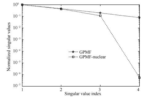
Fig. 1 gives the first four singular values of the matrix ($Y_{0|r-1}^j U_{0|r-1}^{j\bot}$) consisting of the GPMF filtered outputs of the estimated models,where the singular values are normalized by the maximum singular value. As seen clearly from the figure,for Example 1,the singular values of ($Y_{0|r-1}^j U_{0|r-1}^{j\bot}$) from the GPMF method are very close to each other,which makes the determination of model order difficult. In contrast,the singular values from NNM GPMF algorithm show a significant difference at the fourth singular value,which makes the determination of order easier.

|
Download:
|
| Fig. 1. Singular values of the Hankel matrices from GPMF and NNM GPMF algorithms for Example 1. | |
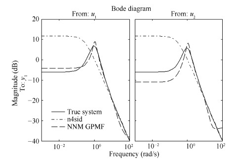
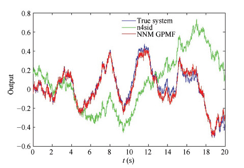
Fig. 2 compares the magnitudes of frequency response of the true system and the estimated models with algorithms n4sid and NNM GPMF,the general GPMF SIM is ignored due to the non-convergent result. As shown in Fig. 2,NNM GPMF algorithm matches best with the true system no matter the frequency is low or high. Fig. 3 compares the noise free output of the true system (47) and the outputs of the models identified by n4sid and NNM GPMF. As seen from the plots,NNM GPMF algorithm outperforms the n4sid and GPMF algorithms significantly in the precision of system identification.

|
Download:
|
| Fig. 2. The magnitude of frequency responses of Example 1. | |

|
Download:
|
| Fig. 3. The system outputs of Example 1. | |
Example 2.
| $\begin{array}{l} \left[ {\begin{array}{*{20}{c}} {{{\dot x}_1}}\\ {{{\dot x}_2}}\\ {{{\dot x}_3}} \end{array}} \right] = \left[ {\begin{array}{*{20}{c}} 0&0&{10}\\ 0&{ - 0.1}&{ - 10}\\ { - 1}&1&{0} \end{array}} \right]\left[ {\begin{array}{*{20}{c}} {{x_1}}\\ {{x_2}}\\ {{x_3}} \end{array}} \right] + \left[ {\begin{array}{*{20}{c}} 1&1&1\\ 2&1&3\\ 1&2&{0} \end{array}} \right]u,\\ \;\;\;\;\;\;\;\;\;\;\;\;\;\;\;\;\;\;y = \left[ {\begin{array}{*{20}{c}} 0&2&{0} \end{array}} \right]\left[ {\begin{array}{*{20}{c}} {{x_1}}\\ {{x_2}}\\ {{x_3}} \end{array}} \right]. \end{array}$ | (48) |
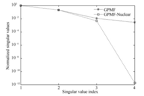
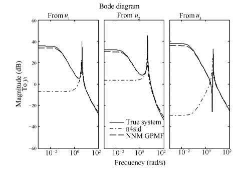
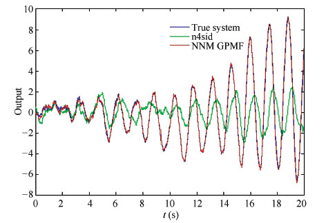
This example is of the same order as Example 1 but with 3-input and 1-output for further assessment of the performance of NNM GPMF. The results of the model order estimations,output errors and validation errors of the three algorithms for this example are shown in Table Ⅰ. As seen from the table,the baseline algorithms n4sid and GPMF give an underestimated model order,2,and larger identification and validation errors than those from the proposed NNM GPMF algorithm. The first four singular values of the matrix ($Y_{0|r-1}^j U_{0|r-1}^{j\bot}$) are given in Fig. 4. The magnitudes of frequency response and outputs of the true system and the models of n4sid and NNM GPMF algorithms are respectively given in Figs. 5 and 6,and the result of GPMF SIM is not convergent as well. Again,the proposed NNM GPMF algorithm performs best.

|
Download:
|
| Fig. 4. Singular values of the Hankel matrices from GPMF and NNM GPMF algorithms for Example 2. | |

|
Download:
|
| Fig. 5. The magnitudes of frequency responses of Example 2. | |

|
Download:
|
| Fig. 6. The system outputs of Example 2. | |
A novel method has been presented for the subspace identification of CT systems. This method incorporates the recently developed NNM technique into the conventional GPMF-based CSIM. It takes the advantage of GPMF algorithm to avoid the time-derivatives of input and output measurements and exploits the power of NNM to minimize the rank of Hankel matrix consisting of the GPMF filtered input and output measurements. An ADMM based computation algorithm has been derived to implement this novel method,and two numerical examples have been presented to verify the validity and evaluate the performance of the proposed method. The examples have demonstrated that the proposed method is superior to the existing methods for CT subspace system identification.
| [1] | Bastogne T, Garnier H, Sibille P. A PMF-based subspace method for continuous-time model identification. Application to a multivariable winding process. International Journal of Control, 2001, 74(2): 118-132 |
| [2] | Rao G P, Unbehauen H. Identification of continuous-time systems. IEE Proceedings: Control Theory and Applications, 2006, 153(2): 185-220 |
| [3] | Campi M C, Sugie T, Sakai F. An iterative identification method for linear continuous-time systems. IEEE Transactions on Automatic Control, 2008, 53(7): 1661-1669 |
| [4] | Cheng C, Wang J D. Identification of continuous-time systems in closedloop operation subject to simple reference changes. In: Proceedings of the 2011 International Symposium on Advanced Control of Industrial Processes (ADCONIP). Hangzhou, China, 2011. 363-368 |
| [5] | Maruta I, Sugie T. Identification of linear continuous-time systems based on the signal projection. In: Proceedings of the 48th IEEE Conference on Decision and Control. Shanghai, China: IEEE, 2009. 7244-7249 |
| [6] | Garnier H, Mensler M, Richard A. Continuous-time model identification from sampled data: implementation issues and performance evaluation. International Journal of Control, 2003, 76(13): 1337-1357 |
| [7] | Garnier H, Sibille P, Richard A. Continuous-time canonical state-space model identification via Poisson moment functionals. In: Proceedings of the 34th IEEE Conference on Decision and Control. .New Orleans, LA: IEEE, 1995 3004-3009 |
| [8] | Prasada R G, Saha D C, Rao T M, Aghoramurthy K, Bhaya A. A microprocessor-based system for on-line parameter identification in continuous dynamical systems. IEEE Transactions on Industrial Electronics, 1982, IE-29(3): 197-201 |
| [9] | Garnier H, Sibille P, Mensler M, Richard A. Pilot crane identification and control in presence of friction. In: Proceedings of the 13th IFAC World Congress. San Francisco, USA: IFAC, 1996. 107-112 |
| [10] | Liu Z, Vandenberghe L. Interior-point method for nuclear norm approximation with application to system identification. SIAM Journal on Matrix Analysis and Applications, 2009, 31(3): 1235-1256 |
| [11] | Falck T, Suykens J A K, Schoukens J, De Moor B. Nuclear norm regularization for overparametrized Hammerstein systems. In: Proceedings of the 49th IEEE Conference on Decision and Control (CDC). Atlanta, GA, USA: IEEE, 2010. 7202-7207 |
| [12] | Fazel M, Pong T K, Sun D F, Tseng P. Hankel matrix rank minimization with applications to system identification and realization. SIAM Journal on Matrix Analysis and Applications, 2011, 34(3): 946-977 |
| [13] | Dvijotham K, Fazel M. A nullspace analysis of the nuclear norm heuristic for rank minimization. In: Proceedings of the 2010 IEEE International Conference on Acoustics, Speech, and Signal Processing (ICASSP). Dallas, TX: IEEE, 2010. 3586-3589 |
| [14] | Ayazoglu M, Sznaier M. An algorithm for fast constrained nuclear norm minimization and applications to systems identification. In: Proceedings of the 2012 IEEE Annual Conference on Decision and Control (CDC). Maui, HI: IEEE, 2012. 3469-3475 |
| [15] | Mohan K, Fazel M. Reweighted nuclear norm minimization with application to system identification. In: Proceedings of the 2010 American Control Conference (ACC). Baltimore, MD: IEEE, 2010. 2953-2959 |
| [16] | Fazel M, Hindi H, Boyd S P. A rank minimization heuristic with application to minimum order system approximation. In: Proceedings of the 2001 American Control Conference. Arlington, VA: IEEE, 2001. 4734-4739 |
| [17] | Hansson A, Liu Z, Vandenberghe L. Subspace system identification via weighted nuclear norm optimization. In: Proceedings of the 2012 IEEE Annual Conference on Decision and Control. Maui, HI: IEEE, 2012. 3439-3444 |
| [18] | Smith R S. Nuclear norm minimization methods for frequency domain subspace identification. In: Proceedings of the 2012 American Control Conference (ACC). Montreal, QC: IEEE, 2012. 2689-2694 |
| [19] | Young P. Parameter estimation for continuous-time models-a survey. Automatica, 1981, 17(1): 23-39 |
| [20] | Garnier H, Wang L P. Identification of Continuous-Time Models from Sampled Data. London: Springer, 2008. |
| [21] | Katayama T. Subspace Methods for System Identification. London: Springer, 2005. |
| [22] | Chen H F. Pathwise convergence of recursive identification algorithms for Hammerstein systems. IEEE Transactions on Automatic Control, 2004, 49(10): 1641-1649 |
| [23] | Mercere G, Ouvrard R, Gilson M, Garnier H. Subspace based methods for continuous-time model identification of MIMO systems from filtered sampled data. In: Proceedings of the 2007 European Control Conference (ECC). Kos: IEEE, 2007.4057-4064 |
| [24] | Greub W. Linear mappings of inner product spaces. Linear Algebra (vol. 23). New York: Springer, 1975. 216-260 |
| [25] | Boyd S, Parikh N, Chu E, Peleato B, Eckstein J. Distributed optimization and statistical learning via the alternating direction method of multipliers. Foundations and Trends°R in Machine Learning, 2011, 3(1): 1-122 |