 2016, Vol.3


2. Department of Mathematics, School of Sciences, Tianjin University, Tianjin 300072, China;
3. Department of Engineering, Peking University, Beijing 100871, China
IN recent years,there has been an increasing number of researches in coordination control of multi-agent systems. Information consensus has attracted more and more attentions in many engineering application fields,such as formation control,flocking, artificial intelligence,automatic control,and so on[1, 2, 3, 4]. A critical problem in distributed control is to develop distributed protocols under which agents can reach an agreement on a common decision.
Convergence rate is an important criterion to evaluate the performance of consensus,which has attracted great attention[5, 6, 7, 8]. In [5],the authors pointed out that the second smallest eigenvalue of its Laplacian matrix was a measure of speed to solve consensus problems. Reference [6] proved that the convergence was sped up by finding the optimal weight associated with each communication link,but the global structure of the network must be known beforehand. Reference [7] accelerated the convergence rate by using the polynomial filtering algorithms. In [8],the authors presented randomized gossip algorithm on an arbitrary connected network and showed its performance precisely in terms of the second largest eigenvalue of an appropriate stochastic matrix. The above literatures all tried to seek a suitable topology communication to achieve fast convergence. In fact,an excellent protocol can reduce cost,increase efficiency and can optimize performance. In practice,it is more useful to design a protocol to obtain better convergence performance under a given topology. In order to get a better convergence speed without changing the topology and edge weights,the authors in [9] proposed a protocol in an unchanged topology network where each node got its state value updated using the information of multi-hop communication for the first time. Then,in [10] the authors discussed that the node in the network topology updated its current state value not only from its immediate neighbors,but also from its second-order neighbors in both discrete-time case and continuous-time case. Further,the authors in [11] extended the systems to second-order case,and made comparisons between the convergence rates of second-order neighbor protocol and a general case. What's more,the delay margins of general protocol and second-order neighbor protocol were derived.
The methods in the papers mentioned above are mainly considered under the traditional time-triggered control actuation schemes. However,since the microprocessor or controller equipped in each agent may have limited resources or energies in practical applications,it is better for the agents to update their control actuation as little frequently as possible. In [12, 13, 14, 15],the authors presented preliminary results of control synthesis for systems with event-based schemes,where the controllers were designed to ensure stability of the closed-loop systems with respect to measurement errors. Many established results referring to event-triggered schemes are in the framework of continuous-time systems,and some of the results have been extended to discrete-time systems[16]. Reference [17] investigated the consensus problem of discrete-time heterogeneous multi-agent systems,where single-integrator and double-integrator agents were explored under distributed event-based control.
Furthermore,most of the above works are based on condition of perfect communication link. However,in reality,the agents exchange data over fading communication channels instead of ideal ones. In fact,in many practical applications,data exchange between sensors is done by wireless communication,which may have a problem of packets losses. Thereby,the packet losses should be taken into account. Many related works have been reported. Reference [18] compared the memory and memoryless consensus protocols in the presence of uniform packet losses. In [19, 20],the authors discussed the average~ consensus~ for the first-order agents and analyzed the convergence speed under data losses. Furthermore,[21] showed that packet dropout could be treated as an absence of a communication link over time. In addition, [22, 23, 24] studied stochastic consensus when each edge of the topology was subject to a random process. On the other hand,communication delays are also instable factors which degrade the performance of the closed-loop systems in various industry processes. Thereby,the study of time-delay systems has attracted considerable attention over the past years. Reference [25] investigated the problem of accelerating average consensus in undirected and connected networks with communication delays for continuous time systems. Discrete systems were extended in [26]. Reference [27] studied the consensus problem of a set of discrete-time heterogeneous multi-agent systems with random communication delays. Furthermore,[28] dealt with consensus with random delay and data losses.
Inspired by the above references,the existing works that use the event-triggered communication scheme such as [16] and [17] only focus on the consensus problem without a leader. In this paper,we consider event-triggered control for leader-follower multi-agent systems with the problem of packet losses and time-varying delays based on second-order neighbors' information. We construct a group of agents,which can communicate with their second-order neighbors and each communication link has a probability of failure. We assume that all channels are independent and subject to a distributed random process,which have the same probability of data loss and time-varying delay. Each agent is equipped with a sampler and a zero-order hold,which are synchronized. Then,by converting the system to the equivalent error dynamics,stochastic stability of the error dynamic system is studied. Here,a Lyapunov function is constructed and a sufficient condition is established to guarantee the event-based mean square consensus in the form of a matrix inequality.
The main contribution of this work is to develop a basic event-triggered tracking control using second-order neighbors' information rather than that of the first-order. Moreover,the time-varying delays and data losses are explicitly taken into account. It differs from the previous work in such aspects: [11] and [13] only focus on the effect of the delay,while we focus more on the failure of links among agents with a probability. Besides, event-triggered tracking control considered in this paper can save agents' energy. Instead of using protocol with first-order information like [21] and [28],we develop the protocol with second-order neighbors' information to accelerate convergence speed.
The rest of this paper is organized as follows. Section Ⅱ provides some preliminaries on graph theory and gives the designed protocol. The main result of this paper is given in Section Ⅲ. Section Ⅳ includes some numerical examples. Finally,Section Ⅴ offers the concluding remarks.
Notation.The set of real numbers is denoted by ${\bf R}$. For any matrix $Q\in{\bf R}^{n\times n}$,sym$(Q)=Q+Q^{\rm T}$. The index set $\Lambda_n$ $=$ $\{1,2,\ldots,n\}$ is a group of consecutive integers from $1$ to $n$. The vector $\textbf{1}_n=[1,1,\ldots,1]^{\rm T}\in{\bf R}^{n}$ has all of its elements equal to 1. The mathematical expectation is denoted by $\mathrm{E}\{\cdot\}$,and $\mathrm{P}\{\cdot\}$ is the probability operator.
Ⅱ. PROBLEM FORMATION A. Preliminaries on Graph TheoryIn this paper,the interaction among $N$ agents is modeled by an undirected graph $G=(V,\varepsilon,A)$,where $V=\{1,2,\ldots, n\}$ is the node set. The edge set $\varepsilon\subseteq V\times V$ contains ordered pairs of nodes. The neighbor set of agent $i$ is denoted as $N_i$,which includes agents from which agent $i$ receives information. The adjacency matrix $A=[w_{ij}]\in{\bf R}^{n \times n}$,is a nonnegative matrix,where $w_{ij}>0$ if and only if edge $(j,i)\in \varepsilon$; otherwise,$w_{ij}$ $=$ $0$. We assume that there is no self-loop,so $w_{ii}=0$. The Laplacian matrix $L=[l_{ij}]\in{\bf R}^{n \times n}$ is defined as
| $ l_{ij}=-w_{ij},\quad {\rm if} ~ i\neq j;\ l_{ii}=\sum\limits_{k\in N_{i}}w_{ik}. $ | (1) |
From the above definitions,we know some facts: $A$ and $L$ determine each other uniquely,and $L$ has nonnegative eigenvalues. Moreover,$L$ has at least one zero eigenvalue with the associated eigenvector $\textbf{1}_n$ $(L\textbf{1}_n=0)$,i.e., span$\{\textbf{1}_n\}\subseteq$ null$\{L\} $,where null$\{L\}$ is the null space of $L$. For the undirected graph,we further have $L=L^{\rm T}$,$\textbf{1}_n^{\rm T}L=0 $. From [29],it is known that span$\{\textbf{1}_n\}={\rm null}\{L\} $ if and only if the undirected graph $G$ is connected.
B. System DynamicsThe dynamics of the $i$-th follower is described as follows:
| $ x_{i}(k+1)=x_{i}(k)+u_{i}(k),~~~i\in\Lambda_{n}, $ | (2) |
where $x_{i}(k)\in{\bf R}$ and $u_{i}(k)\in{\bf R}$ are the position and control input of agent $i$,respectively. The dynamical behavior of active leader is described as follows:
| $ x_{0}(k+1)=x_{0}(k)+v_{0}(k),\notag\\[1mm] v_{0}(k+1)=v_{0}(k)+u_{0}(k), $ | (3) |
where $x_{0}(k),v_{0}(k)\in{\bf R}$ and $u_{0}(k)\in{\bf R}$ are, respectively,the position,velocity,and acceleration of the leader.
Since only the position of the leader can be measured,each follower has to collect information from its neighbors and estimate the leader's velocity during the motion process. A distributed observer-based dynamic tracking control is proposed for each follower $i$:
| $ u_{i}(k)= -c\bigg[\sum\limits_{j\in N_{i}}w_{ij}(x_{i}(k)-x_{j}(k))+b_{i}(x_{i}(k)\notag\\[1mm] -x_{0}(k))\bigg]+v_{i}(k),\notag\\[2mm] v_{i}(k+1)=\ v_{i}(k)+u_{0}(k)-cr\bigg[\sum\limits_{j\in N_{i}}w_{ij}(x_{i}(k)-x_{j}(k))\notag\\[1mm] +b_{i}(x_{i}(k)-x_{0}(k))\bigg], $ | (4) |
where $N_{i}$ is the set consisting of agent $i$'s neighbor agents,$c$ and $r$ are positive scalars. Note that $u_{i}(k)$ in (4) is a local controller of agent $i$,which only depends on the information from its neighbors.
Assumption 1. The time-varying delays are bounded, i.e.,$0\leq d(k)\leq d_{m}$,where $d_{m}$ is a positive scaler.
For the protocol based on second-order neighbors' information, time-varying delays among agents as well as data losses are taken into account in this paper. The following control protocol is adopted:
| $u_{i}(k)= -c\bigg\{\sum\limits_{j\in N_{i}}\gamma_{ij}(k)w_{ij}[(x_{i}(k)-x_{j}(k))\notag\\ +\sum\limits_{h\in N_{j}}\gamma_{jh}(k)w_{jh}(x_{i}(k-d(k))-x_{h}(k-d(k)))]\notag\\ +\gamma_{i0}(k)b_{i}(x_{i}(k)-x_{0}(k))\bigg\}+v_{i}(k),\\ v_{i}(k+1)=\ v_{i}(k)+u_{0}(k)-cr\bigg\{\sum\limits_{j\in N_{i}}\gamma_{ij}(k)w_{ij}[(x_{i}(k)\notag \\ -x_{j}(k))+\sum\limits_{h\in N_{j}}\gamma_{jh}(k)w_{jh}(x_{i}(k-d(k))\notag\\ -x_{h}(k-d(k)))]+\gamma_{i0}(k)b_{i}(x_{i}(k)-x_{0}(k))\bigg\}, $ | (5) |
where $\gamma_{ij}$ (or $w_{ij}$) $=1$,if there is no packet loss between agents $i$ and $j$; $\gamma_{ij}$ (or $w_{ij}$) $=0$, otherwise.
At time $k$,the parameter $w_{ij}(k)$ and $b_{i}(k)$ are chosen by
$$ {w_{ij}}(k) = \left\{ \begin{array}{l} {\alpha _{ij}},{\rm{if}}{\rm{agent}}i{\rm{is}}{\rm{connected}}{\rm{to}}{\rm{agent}}j,\\ 0,{\rm{otherwise,}} \end{array} \right. $$ $$ b_{i}(k)=\begin{cases} \beta_{i},{\rm if\ agent}\ i\ {\rm is \ connected \ to\ the \ leader},\\ 0,\hbox{otherwise}, \end{cases} $$where $\alpha_{ij}>0$ is the connection weight between agent $i$ and agent $j$,and $\beta_{i}>0$ is the connection weight constant between agent $i$ and leader.
Furthermore,we assume that the occurrence of packet loss is governed by a Bernoulli process with uniform probability $p$ satisfying $0<p<1$,i.e.,
| $ P\{\gamma_{ij}(k)=1\}=p,\ P\{\gamma_{ij}(k)=0\}=1-p, \quad\forall i\neq j. $ | (6) |
As a result,we have $\mathrm{E}\{\gamma_{ij}(k)\}=p $.
The undirected topology is coupled,i.e.,for any pair of agents $i$ and $j$,the communication channel between them exists or vanishes simultaneously so that the states of agents can be retained during dynamic evolution.
We define several set of matrices as follows: $L_{1}(k)=$ $[l_{1ij}(k)]\in{\bf R}^{n \times n}$,$L_{2}(k)=[l_{2ij}(k)]\in{\bf R}^{n \times n}$ and $B(k)=$ $[b_{i0}(k)]\in{\bf R}^{n \times n}$, where
$$ l_{1ij}(k)=-\gamma_{ij}(k)w_{ij},\\[1mm] l_{2ij}(k)=-\sum\limits_{h\in N_{i},\ \ j\in N_{h}}\gamma_{ih}(k)w_{ih}\gamma_{hj}(k)w_{hj},i\neq j,\\[1mm] l_{1ii}(k)=\sum\limits_{j\in N_{i}}\gamma_{ij}(k)w_{ij},\\[1mm] l_{2ii}(k)=\sum\limits_{h\in N_{i}}\gamma_{ih}(k)w_{ih}\sum\limits_{l\in N_{h}}\gamma_{hl}(k)w_{hl}, $$and
$$ b_{i0}(k)=\mathrm{diag}\{\gamma_{10}(k)b_{1},\ldots, \gamma_{n0}(k)b_{n}\}. $$As we know,the time-triggered communication scheme as in (5) may produce many useless messages communicated through the network,which then leads to a conservative usage of the communication bandwidth. In order to save the communication energy of the multi-agent network,the event-triggered scheme introduced below realizes the consensus controller (5),where the events are triggered for each agent $i$ when some trigger function is positive.
In the event-triggered cooperative control strategy,suppose $k_{0}^{i},$ $k_{1}^{i},$ $\ldots,$ $k_{l}^{i},$ $\ldots $ is the sequence of the event time of agent $i$ which is defined based on the event-triggered condition. We define the state measurement error by
| $ e_{i}(k)= \hat {x}_{i}(k)-{x}_{i}(k), $ | (7) |
where $\hat {x}_{i}$ is the latest broadcast state of agent $i$ which is given by $\hat {x}_{i}(k)={x}_{i}(k_{l}^{i})$,$k\in [k_{l}^{i},k_{l+1}^{i}).$ Denote $e(k)$ $=[e_{1}(k), e_{2}(k),\ldots,e_{n}(k)]^{\rm T}$,$x(k)=[x_{1}(k),x_{2}(k), \ldots,$ $x_{n}(k)]^{\rm T}$, $\bar{x}(k)=x(k)-x_{0}(k)\textbf{1}_{n},$ then the event-triggered function is defined as
| $ f(\cdot)=\|e(k)\|_{2}^{2}- \sigma \|\bar{x}(k)\|_{2}^{2}, $ | (8) |
where $\sigma$ is a given positive scalar satisfying $0<\sigma<1$ ($i$ $\in$ $\Lambda_{n}$). It should be noted that the state is triggered as soon as the condition (8) is broken.
Then controller (5) under the event-triggered communication scheme can be described as
| $ u_{i}(k)= -c\bigg\{\sum\limits_{j\in N_{i}}\gamma_{ij}(k)w_{ij}[(\hat{x}_{i}(k)-\hat{x}_{j}(k))\notag\\ +\sum\limits_{h\in N_{j}}\gamma_{jh}(k)w_{jh}(\hat{x}_{i}(k-d(k))-\hat{x}_{h}(k-d(k)))]\notag\\ +\gamma_{i0}(k)b_{i}(x_{i}(k)-x_{0}(k))\bigg\}+v_{i}(k),\\ v_{i}(k+1)=\ v_{i}(k)+u_{0}(k)-cr\bigg\{\sum\limits_{j\in N_{i}}\gamma_{ij}(k)w_{ij}[(\hat{x}_{i}(k)\notag\\ -\hat{x}_{j}(k))+\sum\limits_{h\in N_{j}}\gamma_{jh}(k)w_{jh}(\hat{x}_{i}(k-d(k))\notag\\ -\hat{x}_{h}(k-d(k)))]+\gamma_{i0}(k)b_{i}(x_{i}(k)-x_{0}(k))\bigg\}. $ | (9) |
It is noted that both $u_{i}(k)$ and $v_{i}(k)$ use the broadcasted measurements from neighboring followers and from the leader.
Denote vectors $v(k)$ and $u(k)$ by
$$ v(k)=[v_{1}(k),v_{2}(k),\ldots,v_{n}(k)]^{\rm T},\\[1mm] u(k)=[u_{1}(k),u_{2}(k),\ldots,u_{n}(k)]^{\rm T}. $$Then systems (2) and (3) with protocol (9) under the event-triggered communication scheme can be written as
| $ x(k+1)=\ x(k)-cL_{1}(k)x(k)-cL_{2}(k)x(k-d(k))\notag\\[1mm] -cB(k)x(k)+cB(k)\textbf{1}_{n}x_{0}(k)\notag\\[1mm] +v(k)-cL_{1}(k)e(k)-cL_{2}(k)e(k-d(k)),\\ v(k+1)=\ v(k)+u_{0}(k)\textbf{1}_{n}-crL_{1}(k)x(k)\notag\\[1mm] -crL_{2}(k)x(k-d(k))-crB(k)x(k)\notag\\[1mm] +crB(k)\textbf{1}_{n}x_{0}(k) -cL_{1}(k)e(k)\notag\\[1mm] -cL_{2}(k)e(k-d(k)). $ | (10) |
By taking the mathematical expectation of $B(k)$,$ L_{1}(k)$ and $L_{2}(k)$,we have $\mathrm{E}\{B(k)\}=p\times B^{(0)}$, $\mathrm{E}\{L_{1}(k)\}=p\times L^{(1)}$, $\mathrm{E}\{L_{2}(k)\}=p^{2}\times L^{(2)}$,where $B^{(0)}$ is a diagonal matrix representing the leader-follower adjacency relationship where there is no packet loss,$L^{(1)}$ is the nominal Laplacian matrix of full weights where there is no packet loss,and $L^{(2)}$ is the nominal Laplacian matrix of the system which is only based on the second-order neighbors' information with full weights and without packet loss.
Ⅲ. CONVERGENCE ANALYSISDenote $\bar{v}(k)=v(k)-v_{0}(k)\textbf{1}_{n}$,and let $H(k)=L_{1}(k)+B(k)$. Due to $L(k)\times x(k)= L(k)\times \bar{x}(k)$,we have
| $ \bar{x}(k+1)=\ (I_{n}-cH(k))\bar{x}(k)-cL_{2}(k)\bar{x}(k-d(k))\notag\\[1mm] +\bar{v}(k)-cL_{1}(k)e(k)-cL_{2}(k)e(k-d(k)),\notag\\[2mm] \bar{v}(k+1)=\ \bar{v}(k)-crH(k)\bar{x}(k)-crL_{2}(k)\bar{x}(k-d(k))\notag\\[1mm] -crL_{1}(k)e(k)-crL_{2}(k)e(k-d(k)), $ | (11) |
or
| $ \varepsilon(k+1)=F_{1}\varepsilon(k)+F_{2}\varepsilon(k-d(k))+J\epsilon(k), $ | (12) |
where
$$ \varepsilon(k)=\left[\begin{array}{cc} \bar{x}(k)\\ \bar{v}(k) \end{array}\right],\ \ \epsilon(k)=\left[\begin{array}{cc} e(k)\\ e(k-d(k)) \end{array}\right],\\ F_{1}=\left[\begin{array}{cc} I_{n}-cH(k)I_{n}\\ -crH(k)I_{n} \end{array}\right],\ \ F_{2}=\left[\begin{array}{cc} -cL_{2}(k)0\\ -crL_{2}(k)0 \end{array}\right],\\ J=\left[\begin{array}{cc} -cL_{1}(k)-cL_{2}(k)\\ -crL_{1}(k)-crL_{2}(k) \end{array}\right]. $$Before presenting the main results,the following lemma and definition are introduced,which play an important role in the stability analysis of (12).
Definition 1. The system in (12) is said to be mean square stable if
$$ \lim\limits_{m\rightarrow\infty}\mathrm{E}\{\|\bar{x}(m)\|^{2}\}=0,\\[1mm] \lim\limits_{m\rightarrow\infty}\mathrm{E}\{\|\bar{v}(m)\|^{2}\}=0.\\ $$Lemma 1. From above,we can get the following conditions:
$$ \mathrm{E}(\sum\limits_{j\in N_{i}}\gamma_{ij}w_{ij}\times \sum\limits_{j\in N_{i}}\gamma_{ij}w_{ij})\\ \qquad =p\times \sum\limits_{f=1}^{n}\sum\limits_{g=1}^{n}w_{fg}^{2} +p^{2}\times \sum\limits_{f=1}^{n}\sum\limits_{g=1}^{n}\sum\limits_{m=1}^{n}\sum\limits_{s=1}^{n}(w_{fg}w_{ms}),\\ \mathrm{E}(\sum\limits_{h\in N_{i}}\gamma_{ih}w_{ih}\sum\limits_{l\in N_{h}}\gamma_{hl}w_{hl}\times \sum\limits_{h\in N_{i}}\gamma_{ih}w_{ih}\sum\limits_{l\in N_{h}}\gamma_{hl}w_{hl}) \\ =\ p^{2}\times \sum\limits_{f=1}^{n}\sum\limits_{g=1}^{n}\sum\limits_{m=1}^{n}(w_{fg}w_{gm}) \\[1mm] +p^{3}\times \sum\limits_{f=1}^{n}\sum\limits_{g=1}^{n}\sum\limits_{m=1}^{n}\sum\limits_{s=1}^{n}(w_{fg}^{2}w_{gm}w_{gs})\\[1mm] +p^{3}\times \sum\limits_{f=1}^{n}\sum\limits_{g=1}^{n}\sum\limits_{m=1}^{n}\sum\limits_{s=1}^{n}(w_{fg}w_{gm}^{2}w_{sg})\\[1mm] +p^{4}\times \sum\limits_{f=1}^{n}\sum\limits_{g=1}^{n}\sum\limits_{m=1}^{n}\sum\limits_{s=1}^{n}\sum\limits_{u=1}^{n}\sum\limits_{v=1}^{n} (w_{fg}w_{gm}w_{mu}w_{uv}). $$The last equation is to calculate the diagonal entries of $\mathrm{E}\{(L_{1}(k)+L_{2}(k))^{\rm T}Q( L_{1}(k)+L_{2}(k))\} $, which can be extended to the calculation of its off-diagonal entries. Then for an undirected graph,given the Laplacian matrix $B(k)$,$L_{1}(k)$,$L_{2}(k) $ and a symmetric matrix $Q$, $\mathrm{E}\{ B(k)QB(k)\} $ can be calculated as follows
$$ \mathrm{E}\{B(k)QB(k)\}=p^{2}\times B^{(0)}QB^{(0)}+p(1-p)\times \Xi(Q) , $$where $\Xi(Q)$ is a function of $Q$,defined as
$$ \Xi(Q)=\sum\limits_{m=1}^{n}\sum\limits_{q=1}^{n}E^{\rm T}_{(m,m)}QE_{(m,m)}(w_{mq})^{2}. $$In the last equation,$E_{(m,m)}\in {\bf R}^{n\times n}$ has only one nonzero entry equal to 1 at the position $(m,m)$ and all other entries are zero.
And then,
$$ (L^{(1)}+L^{(2)})^{\rm T}Q(L^{(1)}+L^{(2)}) = \left[\begin{array}{ccc} A_{11}\cdots_{1n}\\ \vdots\ddots\vdots\\ A_{n1}\cdots_{nn}\end{array}\right]_{n\times n}, $$where
$$ L(k)=\left[\begin{array}{ccc} \sum\limits_{j\in N_{i}}w_{1j}+\sum\limits_{h\in N_{i}}w_{1h}\sum\limits_{l\in N_{h}}w_{hl}\cdots\\ \vdots\ddots\\ -w_{n1}-w_{n1}\sum\limits_{l\in N_{h}}w_{1l}\cdots\\ \end{array}\right. \\[3mm] \qquad\qquad\qquad\qquad\ \left. \begin{array}{ccc} -w_{1n}-w_{1n}\sum\limits_{l\in N_{h}}w_{nl}\\ \vdots\\ \sum\limits_{j\in N_{i}}w_{nj}+\sum\limits_{h\in N_{i}}w_{nh}\sum\limits_{l\in N_{h}}w_{hl}\end{array}\right]_{n\times n},\\ $$ $$ A_{11}=[(\sum\limits_{j\in N_{i}}w_{1j}+\sum\limits_{h\in N_{i}}w_{1h}\sum\limits_{l\in N_{h}}w_{hl})q_{11}+ \cdots -(w_{1n}\\[1mm] \quad +w_{1n}\sum\limits_{l\in N_{h}}w_{hl})q_{n1}][(\sum\limits_{j\in N_{i}}w_{1j}+\sum\limits_{h\in N_{i}}w_{1h}\sum\limits_{l\in N_{h}}w_{hl})]\\[1mm] \quad + \cdots + [(\sum\limits_{j\in N_{i}}w_{1j}+\sum\limits_{h\in N_{i}}w_{1h}\sum\limits_{l\in N_{h}}w_{hl})q_{1n}\\[1mm] \quad +\cdots-(w_{1n}+w_{1n}\sum\limits_{l\in N_{h}}w_{hl})q_{nn}][-w_{n1}-w_{n1}\sum\limits_{l\in N_{h}}w_{1l}],\\ A_{1n}=[(\sum\limits_{j\in N_{i}}w_{1j}+\sum\limits_{h\in N_{i}}w_{1h}\sum\limits_{l\in N_{h}}w_{hl})q_{11}\\[1mm] \quad +\cdots-(w_{1n}+w_{1n}\sum\limits_{l\in N_{h}}w_{hl})q_{n1}][-w_{1n}-w_{1n}\sum\limits_{l\in N_{h}}w_{nl}]\\[1mm] \quad +\cdots+ [(\sum\limits_{j\in N_{i}}w_{1j}+\sum\limits_{h\in N_{i}}w_{1h}\sum\limits_{l\in N_{h}}w_{hl})q_{1n} +\cdots-(w_{1n}\\[1mm] \quad +w_{1n}\sum\limits_{l\in N_{h}}w_{hl})q_{nn}] [(\sum\limits_{j\in N_{i}}w_{nj}+\sum\limits_{h\in N_{i}}w_{nh}\sum\limits_{l\in N_{h}}w_{hl})],\\[2mm] A_{n1}=[(\sum\limits_{j\in N_{i}}w_{1j}+\sum\limits_{h\in N_{i}}w_{1h}\sum\limits_{l\in N_{h}}w_{hl})q_{11}+ \cdots -(w_{1n}\\[1mm] \quad+w_{1n}\sum\limits_{l\in N_{h}}w_{hl})q_{n1}][(\sum\limits_{j\in N_{i}}w_{1j}+\sum\limits_{h\in N_{i}}w_{1h}\sum\limits_{l\in N_{h}}w_{hl})]\\[1mm] \quad + \cdots + [(\sum\limits_{j\in N_{i}}w_{1j}+\sum\limits_{h\in N_{i}}w_{1h}\sum\limits_{l\in N_{h}}w_{hl})q_{1n}\\[1mm] \quad+\cdots-(w_{1n}+w_{1n}\sum\limits_{l\in N_{h}}w_{hl})q_{nn}][-w_{n1}-w_{n1}\sum\limits_{l\in N_{h}}w_{1l}],\\[2mm] A_{nn}=[(\sum\limits_{j\in N_{i}}w_{1j}+\sum\limits_{h\in N_{i}}w_{1h}\sum\limits_{l\in N_{h}}w_{hl})q_{11}\\[1mm] \quad+\cdots-(w_{1n}+w_{1n}\sum\limits_{l\in N_{h}}w_{hl})q_{n1}][-w_{1n}-w_{1n}\sum\limits_{l\in N_{h}}w_{nl}]\\[1mm] \quad +\cdots+ [(\sum\limits_{j\in N_{i}}w_{1j}+\sum\limits_{h\in N_{i}}w_{1h}\sum\limits_{l\in N_{h}}w_{hl})q_{1n} +\cdots-(w_{1n}\\[1mm] \quad +w_{1n}\sum\limits_{l\in N_{h}}w_{hl})q_{nn}] [(\sum\limits_{j\in N_{i}}w_{nj}+\sum\limits_{h\in N_{i}}w_{nh}\sum\limits_{l\in N_{h}}w_{hl})]. $$Combining $L_{1}(k)$ and $L_{2}(k)$,the calculation of $\mathrm{E}\{(L_{1}(k)+L_{2}(k))^{\rm T}Q( L_{1}(k)+L_{2}(k))\} $ is achieved similarly to that of $(L^{(1)}+L^{(2)})^{\rm T}Q(L^{(1)}+L^{(2)})$. The following theorem gives a sufficient condition on the mean square consensus of the system.
Theorem 1. Given the scalars $r$ and $c$,if there exist matrices $Q>0$,$P>0$,$R>0$,$Z>0$,such that the following matrix inequality holds:
$$ F_{3}=A+W+L<0, $$the mean square consensus of the system (12) is achieved asymptotically under the event-triggered condition with
$$ W=\left[\begin{array}{cccccc} -2cpH^{(0)}+c^{2}\hat{p}_{31}+c^{2}r^{2}\bar{p}_{31}2I_{n}-2cpH^{(0)}-2crpH^{(0)}Q \\ *I_{n}\\ **\\ **\\ **\\ **\\ \end{array}\right. \\[2mm] \left. \begin{array}{cccccc} 2S_{2}02S_{1}2S_{2}\\ -2cpL^{(2)}\!-\!2crpQL^{(2)}0-2cpL^{(1)}\!-\!2crpQL^{(1)}\!\!\!\!-2cpL^{(2)}\!-\!2crpQL^{(2)}\\ c^{2}\hat{p}_{22}+c^{2}r^{2}\bar{p}_{22}02c^{2}\hat{p}_{21}+2c^{2}r^{2}\bar{p}_{21}2c^{2}\hat{p}_{22}+2c^{2}r^{2}\bar{p}_{22}\\ *000\\ **c^{2}\hat{p}_{11}+c^{2}r^{2}\bar{p}_{11}2c^{2}\hat{p}_{12}+2c^{2}r^{2}\bar{p}_{12}\\ ***c^{2}\hat{p}_{22}+c^{2}r^{2}\bar{p}_{22} \end{array}\!\!\!\!\!\right], $$ $$ A=\left[\begin{array}{cccccc} d_{m}c^{2}\hat{p}_{31}+d_{m}c^{2}r^{2}\bar{y}_{31}2d_{m}cpH^{(0)} 2d_{m}S_{4}\\ *d_{m}I_{n}-2d_{m}cpL^{(2)}\\ **d_{m}c^{2}\hat{p}_{22}+d_{m}c^{2}r^{2}\bar{y}_{22}\\ ***\\ ***\\ ***\\ \end{array}\right. \\[1mm] \qquad\qquad\qquad\qquad\left. \begin{array}{cccccc} 02d_{m}S_{3}2d_{m}S_{4}\\ 0-2d_{m}cpL^{(1)}-2d_{m}cpL^{(2)}\\ 02d_{m}c^{2}\hat{p}_{21}+2d_{m}c^{2}r^{2}\bar{y}_{21}2d_{m}c^{2}\hat{p}_{22}+2d_{m}c^{2}r^{2}\bar{y}_{22}\\ 000\\ *d_{m}c^{2}\hat{p}_{11}+d_{m}c^{2}r^{2}\bar{y}_{11}2d_{m}c^{2}\hat{p}_{12}+2d_{m}c^{2}r^{2}\bar{y}_{12}\\ **d_{m}c^{2}\hat{p}_{22}+d_{m}c^{2}r^{2}\bar{y}_{22} \end{array}\right], $$where
$$ \hat{p}_{31}=\ \mathrm{E}(H^{2}(k))=\hat{p}_{11}+2p^{2}B^{(0)}L^{(1)}+pB^{(0)},\\[2mm] \bar{p}_{31}=\ \mathrm{E}(H(k)QH(k))\\ =\ \bar{p}_{11}+p^{2}B^{(0)}QL^{(1)}+p^{2}L^{(1)}QB^{(0)}\\ +p^{2}\times B^{(0)}QB^{(0)}+p(1-p)\times \Xi(Q),\\[2mm] S_{1}=\ \mathrm{E}(-cL_{1}(k)+c^{2}H(k)L_{1}(k)+c^{2}r^{2}H(k)QL_{1}(k))\\= -cpL^{(1)}+c^{2}(\hat{p}_{11}+p^{2}B^{(0)}L^{(1)}\\ +c^{2}r^{2}(\bar{p}_{11}+p^{2}B^{(0)}QL^{(1)},\\[2mm] S_{2}=\ \mathrm{E}(-cL_{2}(k)+c^{2}H(k)L_{2}(k)+c^{2}r^{2}H(k)QL_{2}(k))\\= -cpL^{(2)}+c^{2}(\hat{p}_{12}+p^{2}B^{(0)}L^{(2)})\\ +c^{2}r^{2}(\bar{p}_{12}+p^{2}B^{(0)}QL^{(2)}),\\[2mm] \bar{y}_{31}=\ \mathrm{E}(H(k)ZH(k))=\bar{y}_{11}+p^{2}B^{(0)}ZL^{(1)}\\ +p^{2}L^{(1)}ZB^{(0)}+p^{2}\times B^{(0)}ZB^{(0)}+p(1-p)\times \Xi(Z),\\[2mm] S_{3}=\ \mathrm{E}(c^{2}H(k)L_{1}(k)+c^{2}r^{2}H(k)ZL_{1}(k))\\=\ c^{2}(\hat{p}_{11}+p^{2}B^{(0)}L^{(1)})+c^{2}r^{2}(\bar{y}_{11}+p^{2}B^{(0)}ZL^{(1)}),\\[2mm] S_{4}=\ \mathrm{E}(c^{2}H(k)L_{2}(k)+c^{2}r^{2}H(k)ZL_{2}(k))\\=\ c^{2}(\hat{p}_{12}+p^{2}B^{(0)}L^{(2)})+c^{2}r^{2}(\bar{y}_{12}+p^{2}B^{(0)}ZL^{(2)}),\\[2mm] L=\ \left[\begin{array}{ccc} \Phi+d_{m}M\bar{Z}^{-1}M^{\rm T}00\\ *R-I_{n}0\\ **-R \end{array}\right],\\[2mm] \Phi=\ \left[\begin{array}{cc} M_{1}+M_{1}^{\rm T}+\bar{P}+\Psi-M_{1}+M_{2}\\ *-M_{2}-M_{2}^{\rm T}-\bar{Q}-\bar{P} \end{array}\right],\\[2mm] \Psi=\ \left[\begin{array}{cc} \sigma I_{n}0\\ 00 \end{array}\right], $$and
$$ \bar{p}_{11}=\ \mathrm{E}(L_{1}(k)QL_{1}(k)),\quad \bar{p}_{12}= \mathrm{E}(L_{1}(k)QL_{2}(k)),\\[1mm] \bar{p}_{21}=\ \mathrm{E}(L_{2}(k)QL_{1}(k)),\quad \bar{p}_{22}= \mathrm{E}(L_{2}(k)QL_{2}(k)),\\[1mm] \bar{y}_{11}=\ \mathrm{E}(L_{1}(k)ZL_{1}(k)),\quad \bar{y}_{12}= \mathrm{E}(L_{1}(k)ZL_{2}(k)),\\[1mm] \bar{y}_{21}=\ \mathrm{E}(L_{2}(k)ZL_{1}(k)),\quad \bar{y}_{22}= \mathrm{E}(L_{2}(k)ZL_{2}(k)),\\[1mm] \hat{p}_{11}=\ \mathrm{E}(L_{1}(k)L_{1}(k)),\quad \hat{p}_{12}= \mathrm{E}(L_{1}(k)L_{2}(k)),\\[1mm] \bar{p}_{21}=\ \mathrm{E}(L_{2}(k)L_{1}(k)),\quad \hat{p}_{22}= \mathrm{E}(L_{2}(k)L_{2}(k)). $$Proof. Construct the candidate Lyapunov function as
$$ V(k)=V_{1}(k)+V_{2}(k)+V_{3}(k)+V_{4}(k),\\[1mm] V_{1}(k)=\varepsilon^{\rm T}(k)\bar{Q}\varepsilon(k),\\ V_{2}(k)=\sum\limits_{i=k-d(k)}^{k-1}\varepsilon^{\rm T}(i)\bar{P}\varepsilon(i),\\ V_{3}(k)=\sum\limits_{i=k-d(k)}^{k-1}e^{\rm T}(i)Re(i),\\ V_{4}(k)=\sum\limits_{j=-d_{m}}^{-1}\sum\limits_{i=k+j}^{k-1}\eta^{\rm T}(i)\bar{Z}\eta(i), $$where
$$ \bar{Q}=\left[ \begin{array}{cc} I_{n}0\\ 0Q \end{array}\right], \ \ \bar{P}=\left[ \begin{array}{cc} I_{n}0\\ 0P \end{array}\right], \ \ \bar{Z}=\left[ \begin{array}{cc} I_{n}0\\ 0Z \end{array}\right], $$and in $V_{4}(k)$,$\eta(i)=\varepsilon(i+1)-\varepsilon(i)$. Then from (12) we have
$$ \mathrm{E}\{\Delta V_{1}(k)\}=\mathrm{E}\{V_{1}(k+1)-V_{1}(k)\}\\[1mm] =\mathrm{E}\{\varepsilon^{\rm T}(k+1)\bar{Q}\varepsilon(k+1)-\varepsilon^{\rm T}(k)\bar{Q}\varepsilon(k)\}. $$Using Lemma 1,$\mathrm{E}\{\Delta V_{1}(k)\}$ can be calculated as
$$ \mathrm{E}\{\Delta V_{1}(k)\}=\delta^{\rm T}(k)W\delta(k), $$where $\delta(k)=[\varepsilon^{\rm T}(k)\quad \varepsilon^{\rm T}(k-d(k))\quad \epsilon(k)]^{\rm T}$.
For the second term,
$$ \mathrm{E}\{\Delta V_{2}(k)\}= \mathrm{E}\{V_{2}(k+1)-V_{2}(k)\}\\[1mm] = \varepsilon^{\rm T}(k){\rm Re}\varepsilon(k)-\varepsilon^{\rm T}(k-d(k)){\rm Re}\varepsilon(k-d(k)). $$For the third term,
$$ \mathrm{E}\{\Delta V_{3}(k)\}= \mathrm{E}\{V_{3}(k+1)-V_{3}(k)\}\\[1mm] = e^{\rm T}(k){\rm Re}(k)-e^{\rm T}(k-d(k)){\rm Re}(k-d(k)). $$For the fourth term,
$$ \mathrm{E}\{\Delta V_{4}(k)\}= \mathrm{E}\{V_{4}(k+1)-V_{4}(k)\}\\[1mm] = \mathrm{E} \{\eta^{\rm T}(k)d_{m}\bar{Z}\eta(k)-\sum\limits_{j=k-d_{m}}^{k-1}\eta^{\rm T}(j)\bar{Z}\eta(j)\}\\[1mm] = \delta^{\rm T}(k)A\delta(k)-\sum\limits_{j=k-d_{m}}^{k-1}\eta^{\rm T}(j)\bar{Z}\eta(j). $$Then define
$$ \xi(k)=\left[\begin{array}{cc} \varepsilon(k)\\[1mm] \varepsilon(k-d(k)) \end{array}\right]. $$For any matrix $M=[M_{1}^{\rm T}$,$M_{2}^{\rm T}]^{\rm T}$, $M_{1}$,$M_{2} \in {\bf R}^{2n\times 2n}$,consider the nonnegative term
| $ 0\leq \sum\limits_{j=k-d(k)}^{k-1}[\xi^{\rm T}(k)M+\eta^{\rm T}(j)\bar{Z}]\bar{Z}^{-1}[M^{\rm T}\xi(k)+\bar{Z}\eta(j)]\notag\\[1mm] =\ d(k)\xi^{\rm T}(k)M\bar{Z}^{-1}M^{\rm T}\xi(k) \notag\\[1mm] +2\xi^{\rm T}(k)M\sum\limits_{j=k-d(k)}^{k-1}\eta(j)+\sum\limits_{j=k-d_{k}}^{k-1}\eta^{\rm T}(j)\bar{Z}\eta(j)\notag\\[1mm] \leq\ \xi^{\rm T}(k)(d_{m}M\bar{Z}^{-1}M^{\rm T})\xi(k)+2\xi^{\rm T}(k)M[\varepsilon(k)\notag\\[1mm] -\varepsilon(k-d(k))]+ \sum\limits_{j=k-d_{m}}^{k-1}\eta^{\rm T}(j)\bar{Z}\eta(j)=Y(k). $ | (13) |
Notice that (8) can always guarantee $f(\cdot)\leq 0$,which means
$$ \|e(k)\|_{2}^{2}\leq \sigma \|\bar{x}(k)\|_{2}^{2}. $$Summing up $\mathrm{E}\{\Delta V_{1}(k)\}$,$\mathrm{E}\{\Delta V_{2}(k)\}$,$\mathrm{E}\{\Delta V_{3}(k)\}$,$\mathrm{E}\{\Delta V_{4}(k)\}$ and (13) under event-triggered condition,we obtain that
| $ \mathrm{E}\{\Delta V(k)\}\leq\mathrm{E}\{\Delta V_{1}(k)\}+\mathrm{E}\{\Delta V_{2}(k)\} +\mathrm{E}\{\Delta V_{3}(k)\}\notag\\[1mm] \qquad + \mathrm{E}\{\Delta V_{4}(k)\} +Y(k)+\sigma \bar{x}^{\rm T}(k)\bar{x}(k)-e^{\rm T}(k)e(k)\notag\\[1mm] \qquad = \delta^{\rm T}(k)(A+W+L)\delta(k)=\delta^{\rm T}(k)F_{3}\delta(k)\leq 0. $ | (14) |
Thus,the subsequent task is to show that the error dynamic system is stable in the mean square sense. Let the largest eigenvalue of $F_{3}$ be $\lambda_{\max}$,then
| $ \mathrm{E}\{V(k+1)-V(k)\} \leq \delta^{\rm T}(k)F_{3}\delta(k)\leq \lambda_{\max} \|\delta(k)\|^{2}. $ | (15) |
Summing (15) from $k=0$,we obtain that
$$ \mathrm{E}\{V(k+1)-V(0)\} \leq \lambda_{\max} \sum\limits_{m=0}^{k} \mathrm{E}\{\|\delta(m)\|^{2}\},\\[1mm] \sum\limits_{m=0}^{k} \mathrm{E}\{\|\delta(m)\|^{2}\}\leq -\frac{1}{\lambda_{\max} }\mathrm{E}\{V(0)-V(k+1)\}. $$Let $k\rightarrow \infty$,the following inequality can be derived:
$$ \sum\limits_{m=0}^{k} \mathrm{E}\{\|\delta(m)\|^{2}\} \leq -\frac{1}{\lambda_{\max} }\mathrm{E}\{V(0)-V(\infty)\}\\[1mm] \leq- \frac{1}{\lambda_{\max} }\mathrm{E}\{V(0)\}. $$Considering that $\|\delta(m)\|^{2}\geq \|\bar{x}(m)\|^{2}$, $\|\delta(m)\|^{2}\geq \|\bar{v}(m)\|^{2}$,$m=0,1,2,\ldots$, therefore,
$$ \sum\limits_{m=0}^{k} \mathrm{E}\{\|\bar{x}(m)\|^{2}\}\leq \sum\limits_{m=0}^{k} \mathrm{E}\{\|\delta(m)\|^{2}\}\\[1mm] \qquad \leq- \frac{1}{\lambda_{\max} }\mathrm{E}\{V(0)\}lt;\infty,\\[2mm] \sum\limits_{m=0}^{k} \mathrm{E}\{\|\bar{v}(m)\|^{2}\}\leq \sum\limits_{m=0}^{k} \mathrm{E}\{\|\delta(m)\|^{2}\}\\[1mm] \qquad\leq- \frac{1}{\lambda_{\max} }\mathrm{E}\{V(0)\}lt;\infty. $$Then,it can be concluded that lim$_{m\rightarrow\infty}\mathrm{E}\{\|\bar{x}(m)\|^{2}\}=0$, lim$_{m\rightarrow\infty}\mathrm{E}\{\|\bar{v}(m)\|^{2}\}=0$,and thus the error dynamic system in (12) is mean square stable. So consensus is achieved in the mean square sense.
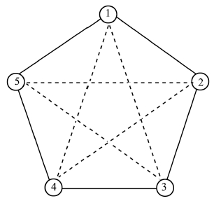
Ⅳ. SIMULATIONSTo illustrate convergence rate of the protocol for the tracking consensus of system (12) based on second-order neighbors' information,one numerical example of leader-follower multi-agent systems is provided. The nominal interaction topology and the topology based on second-order neighbors' information among five agents are shown in Fig. 1.

|
Download:
|
| Fig. 1. Nominal communication topology based on the second-order neighbors' information. | |
The weights are set to be unique for simplicity here. The corresponding Laplacian matrices $L^{(1)}$ and $L^{(2)}$ are given as follows:
$$ L^{(1)}=\left[\begin{array}{rrrrr}2-100-1\\ -12-100\\[1mm] 0-12-10\\[1mm] 00-12-1\\[1mm] -100-12\end{array}\right],\\[2mm] L^{(2)}=\left[\begin{array}{rrrrr}20-1-10\\ 020-1-1\\[1mm] -1020-1\\[1mm] -1-1020\\[1mm] 0-1-102 \end{array}\right], $$and the diagonal matrix for the interconnection relationship between the leader and the followers is:
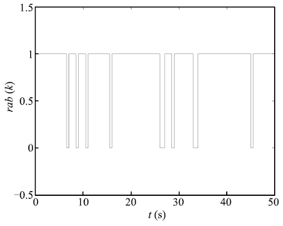
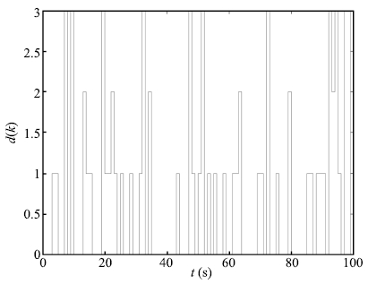
$$ B^{(0)}={\rm diag}\{1,1,1,1,1\}. $$We choose the probability of successfully receiving information as $p=0.9$. The time history of Bernoulli variable $\gamma_{ab}(k)$ is shown in Fig. 2. Fig. 3 is the time delay $d(k)$ that is uniformly distributed between 0 and 3.

|
Download:
|
| Fig. 2. Time history of Bernoulli variable $\gamma_{ab}(k)$. | |

|
Download:
|
| Fig. 3. Time delay $d(k)$ over time. | |
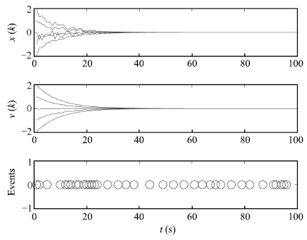
We choose control gain $c=0.3$,$r=0.1$,the triggered parameter $ \sigma=0.54$ and the initial condition $x(0)=[-2,-1,$ $0,1,2]$, $v(0)=[-2, -1, 0, 1, 2]$. Choose the initial position,initial velocity of the leader as $x_{0}(0)=0$,$v_{0}(0)=$ $0$. Let $p$ $\rightarrow$ $1$,by solving the matrix inequality in Theorem 1 we get
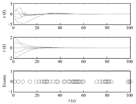
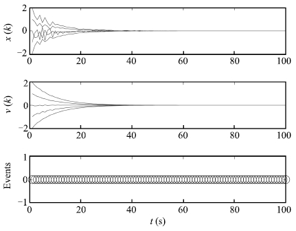
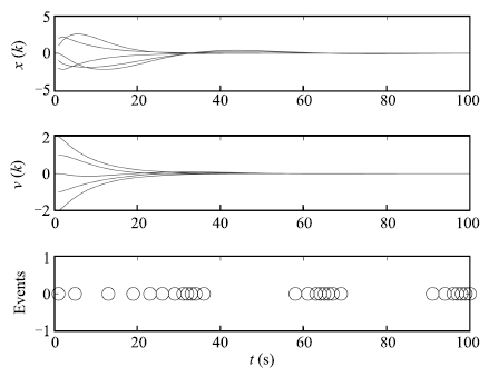
$$ Q=\\[2mm] \ \left[\begin{array}{rrrrr} 7.9191 -1.0690 0.2035-0.3065-1.6245\\[2mm] -1.0690 7.8870 -1.1585 -0.2854 -0.2366\\[2mm] 0.2035 -1.1585 7.8175 -1.1980 -0.3780\\[2mm] -0.3065 -0.2854 -1.1980 7.8867 -1.0266\\[2mm] -1.6245 -0.2366 -0.3780 -1.0266 8.1072\end{array}\right]. $$Thus consensus will be achieved for the system either with or without time delays. Fig. 4 shows the state,velocity trajectories and event times of the agents under protocol (9) when $p=0.9$. Fig. 5 shows the state,velocity trajectories and event times of the agents under protocol (4) when $p=0.9$. From which we know that in this case the system converges faster under protocol (9) than under protocol (4). Fig. 6 shows the simulation results of protocol (5) for $p=0.9$ under time-triggered control strategy. Comparing Fig. 4 and Fig. 6,we know that the system also achieve consensus under event-triggered control,which reduces the number of agent updating times and thus saves the energy. Fig. 7 shows the simulation results of protocol (9) for $ p=0.5$,Comparing Fig. 4 and Fig. 7,we know that the system converges faster under lower probability of packet losses.

|
Download:
|
| Fig. 4. Protocol (9) for $p=0.9$. | |

|
Download:
|
| Fig. 5. Protocol (4) for $p=0.9$. | |

|
Download:
|
| Fig. 6. Protocol (5) for $p=0.9$. | |

|
Download:
|
| Fig. 7. Protocol (9) for $p=0.5$. | |
In this paper,we have investigated the mean square consensus for the leader-follower multi-agent systems with the problem of packet losses and communication delays when second-order neighbors' information are used. The convergence rates of general protocol and second-order neighbor protocol have been compared and it is concluded that second-order neighbor protocol speeds up the consensus rate. What is more,we can see that system converges faster under lower probability of packet losses. Future work will include consensus tracking issue of the second-order multi-agent systems under stochastic switching topology.
| [1] | Su H S, Chen M Z Q, Wang X F, Lam J. Semiglobal observer-based leader-following consensus with input saturation. IEEE Transactions on Industrial Electronics, 2014, 61(6): 2842-2850 |
| [2] | Su H S, Chen M Z Q, Lam J, Lin Z L. Semi-global leader-following consensus of linear multi-agent systems with input saturation via low gain feedback. IEEE Transactions on Circuits and Systems I: Regular Papers, 2013, 60(7): 1881-1889 |
| [3] | He W, Cao J. Consensus control for high-order multi-agent systems. IET Control Theory and Applications, 2011, 5(1): 231-238 |
| [4] | He W L, Han Q L, Qian F. Synchronization of heterogeneous dynamical networks via distributed impulsive control. In: Proceedings of the 40th Annual Conference of the IEEE Industrial Electronics Society. Dallas, TX: IEEE, 2014. 3713-3719 |
| [5] | Olfati-Saber R, Murray R M. Consensus problems in networks of agents with switching topology and time-delays. IEEE Transactions on Automatic Control, 2004, 49(9): 1520-1533 |
| [6] | Xiao L, Boyd S. Fast linear iterations for distributed averaging. Systems and Control Letters, 2004, 53(1): 65-78 |
| [7] | Kokiopoulou E, Frossard P. Polynomial filtering for fast convergence in distributed consensus. IEEE Transactions on Signal Processing, 2009, 57(1): 342-354 |
| [8] | Boyd S, Ghosh A, Prabhakar B, Shah D. Randomized gossip algorithms. IEEE Transactions on Information Theory, 2006, 52(6): 2508-2530 |
| [9] | Jin Z P, Murray R M. Multi-hop relay protocols for fast consensus seeking. In: Proceedings of the 45th IEEE Conference on Decision and Control. San Diego, CA: IEEE, 2006. 1001-1006 |
| [10] | Yuan D M, Xu S Y, Zhao H Y, Chu Y M. Accelerating distributed average consensus by exploring the information of second-order neighbors. Physics Letters A, 2010, 374(24): 2438-2445 |
| [11] | Pan H, Nian X H, Guo L. Second-order consensus in multi-agent systems based on second-order neighbours' information. International Journal of Systems Science, 2014, 45(5): 902-914 |
| [12] | Wang X F, Lemmon M D. Decentralized event-triggered broadcasts over networked control systems. In: Proceedings of the 11th International Workshop. St. Louis, MO, USA: Springer, 2008. 674-677 |
| [13] | Wang X F, Lemmon M. On event design in event-triggered feedback systems. Automatica, 2011, 47(10): 2319-2322 |
| [14] | Zhu W, Jiang Z P. Event-based leader-following consensus of multiagent systems with input time delay. IEEE Transactions on Automatic Control, 2015, 60(5): 1362-1367 |
| [15] | Mu N K, Liao X F, Huang T W. Event-based consensus control for a linear directed multiagent system with time delay. IEEE Transactions on Circuits and Systems II: Express Briefs, 2015, 62(3): 281-285 |
| [16] | Eqtami A, Dimarogonas D V, Kyriakopoulos K J. Event-triggered control for discrete-time systems. In: Proceedings of the 2010 American Control Conference. Baltimore, MD: IEEE, 2010. 4719-4724 |
| [17] | Yin X X, Yue D, Hu S L. Distributed event-triggered control of discretetime heterogeneous multi-agent systems. Journal of the Franklin Institute, 2013, 350(3): 651-669 |
| [18] | Wang S, An C J, Sun X X, Du X. Average consensus over communication channels with uniform packet losses. In: Proceedings of the 2010 Chinese Control and Decision Conference. Xuzhou, China: IEEE, 2010. 114-119 |
| [19] | Fagnani F, Zampieri S. Randomized consensus algorithms over large scale networks. IEEE Journal on Selected Areas in Communications, 2008, 26(4): 634-649 |
| [20] | Fagnani F, Zampieri S. Average consensus with packet drop communication. SIAM Journal of Control and Optimization, 2009, 48(1): 102-133 YU et al.: EVENT-TRIGGERED TRACKING CONSENSUS WITH PACKET LOSSES AND TIME-VARYING DELAYS 173 |
| [21] | Wu J, Shi Y. Average consensus in multi-agent systems with timevarying delays and packet losses. In: Proceedings of the 2012 American Control Conference. Montreal, QC: IEEE, 2012. 1579-1584 |
| [22] | Hatano Y, Mesbahi M. Agreement over random networks. IEEE Transactions on Automatic Control, 2005, 50(11): 1867-1872 |
| [23] | Wu C W. Synchronization and convergence of linear dynamics in random directed networks. IEEE Transactions on Automatic Control, 2006, 51(7): 1207-1210 |
| [24] | Porfiri M, Stilwell D J. Consensus seeking over random weighted directed graphs. IEEE Transactions on Automatic Control, 2007, 52(9): 1767-1773 |
| [25] | Rong L, Xu S Y, Zhang B Y, Zou Y. Accelerating average consensus by using the information of second-order neighbours with communication delays. International Journal of Systems Science, 2013, 44(6): 1181- 1188 |
| [26] | Kapila V, Haddad W M. Memoryless H1 controllers for discrete-time systems with time delay. Automatica, 1998, 34(9): 1141-1144 |
| [27] | Yin X X, Yue D. Event-triggered tracking control for heterogeneous multi-agent systems with Markov communication delays. Journal of the Franklin Institute, 2013, 350(5): 1312-1334 |
| [28] | Zhang Y, Tian Y P. Consensus of data-sampled multi-agent systems with random communication delay and packet loss. IEEE Transactions on Automatic Control, 2010, 55(4): 939-943 |
| [29] | Wei R, Beard R W. Consensus seeking in multiagent systems under dynamically changing interaction topologies. IEEE Transactions on Automatic Control, 2005, 50(5): 655-661 |