2. Hongguang Ma is with Beijing Institute of Technology, Zhuhai 519088, China
NURAL network for principal component analysis (PCA) is an important method for feature extraction and data compression applications. Until now,a significant amount of neural network algorithms for PCA have been proposed. Compared with neural based PCA algorithms,the field of neural network algorithms that perform the singular value decomposition (SVD) received relatively little attention[1]. Actually,neural networks can also provide an effective approach for SVD of rectangular matrix between two data streams[2, 3, 4, 5].
In an earlier time,some methods for SVD were developed by using purely matrix algebra[6, 7, 8, 9],but these methods are batching methods and thus can not be used for real-time processing. To extract feature information online,some SVD dynamical systems based on gradient flows are developed[10, 11, 12],but these algorithms converge slowly. To overcome this problem,Diamantaras and Kung[5] extended the online correlation Hebbian rule to the cross-correlation Hebbian rule to perform the SVD of a cross-correlation matrix. However,the models are sometimes divergent for some initial states[4]. Feng et al. provided a theoretical foundation for a novel model based on an extension of the Hebbian rule[13]. In order to improve the convergence speed and stability,Feng proposed a cross-correlation neural network (CNN) learning rule for SVD[4] in which the learning rate is independent of the singular value distribution of a non-squared data or cross-correlation matrix. It is found that all efforts of aforementioned work are only focused on single singular component analysis. Actually,there are also some principal singular subspace (PSS) extraction algorithms that have been proposed. In [14],a novel CNN model for finding the PSS of a cross-correlation matrix was proposed. Hasan[15] proposed an algorithm to track PSS in which the equilibrium point relates to the principal singular values. Later,Kong et al.[16] proposed an effective neural network algorithm for cross-correlation feature extraction,which is also a parallel algorithm. As known,neural network algorithm for extracting the principal singular vectors/subspace,which is always derived based on Hebbian rule or gradient method,is a special case of optimization problem. Actually,solving the optimization problems by using the recurrent neural network has also been well studied in [17, 18, 19].
In [1],neural network algorithms that only consider the singular vectors extraction are coined as noncoupled algorithms. In most of noncoupled algorithms,the convergence speed depends on the singular values of the cross-covariance matrix,but it is hard to select an appropriate learning rate. This problem was coined as the speed-stability problem[1]. In order to solve this problem, Kaiser et al.[1] proposed a coupled neural network algorithm based on Newton's method,in which the principal singular triplet (PST) is estimated simultaneously.
Coupled learning algorithm,which can control the learning rate of an eigenvector estimate by the corresponding eigenvalue estimate, has favorable convergence properties[1]. Besides singular vectors,CSVD algorithm can also extract the singular values, which are very important and useful in some engineering practice; on the other hand,CSVD algorithm can solve the speed-stability problem which plagues most noncoupled algorithms,and thus converge faster than noncoupled algorithms. But unfortunately, there is only one CSVD algorithm that has been proposed and analyzed so far. In this paper,we successfully derive a new CSVD algorithm based on Kaiser's work. Our work is an improvement and expansion of Kaiser's work.
In this paper,we propose a novel information criterion (NIC),in which the desired solution corresponds to one of the stationary points. The gradient-based method is not suitable for the NIC since the first PST of the NIC is not a minimum but a saddle point. Nevertheless,the learning rule can be derived by applying Newton's method,in this case,the key point is to find the gradient and to approximate the inverse Hessian of the NIC. Then, we obtain an algorithm based on the gradient and the inverse Hessian. Stability of proposed algorithm is analyzed by finding the eigenvalues of the Jacobian of the ordinary differential equations (ODEs). Stability analysis shows that the algorithm solves the speed-stability problem since it converges with approximately equal speed in almost all of its eigen-directions and is widely independent of its singular values. Based on the experiment results,we find that the proposed algorithm converge faster than existing noncoupled algorithms. Compared with noncoupled algorithms,the proposed algorithm can also estimate the principal singular values. In this paper,the approach of approximating the inverse Hessian is different from that in [1]. The information criterion introduced in [1] contains a natural logarithm of singular value,which is not suitable for negative singular value. The proposed information criterion overcomes this weakness.
Ⅱ. PRELIMINARIESLet A denote an $m\times n$ real matrix and its SVD is given by[1]
| $ A=\bar{U}\bar{S}\bar{V}^{\rm T}+\bar{U}_2\bar{S}_2\bar{V}^{\rm T}_2, $ | (1) |
where $\bar{U} \in {\bf R}^{m\times M}$ and $\bar{V} \in {\bf R}^{n\times M}$ ($M\leq \text{min}\{m,n\}$) denote the left and right PSS of $A$,respectively. And $\bar{U} = [\bar{{u}}_1,\ldots,\bar{{u}}_M]$ and $\bar{V} = [\bar{{v}}_1,\ldots,\bar{{{v}}}_M]$,where $\bar{{u}}_i$ and $\bar{{v}}_i$ ($i=1,\ldots,M$) are the $i$-th left and right principal singular vectors of $A$,respectively. Moreover,$\bar{S} = \text{diag}{\bar{\sigma}_1,\ldots,\bar{\sigma}_M} \in {\bf R}^{M\times M}$ denotes the matrix with the principal singular values on its diagonal. We refer to these matrices as the principal portion of the SVD. $(\bar{{u}}_j,\bar{{v}}_j,\bar{\sigma}_j)$ is called the jth singular triplet of the cross-covariance matrix $A$. Furthermore,$\bar{U}_2 = [\bar{{u}}_{M+1},\ldots,\bar{{u}}_N] \in {\bf R}^{m\times (N-M)}$, $\bar{S}_2 = \text{diag}{\bar{\sigma}_{M+1},\ldots,\bar{\sigma}_N}\in{\bf R}^{(N-M)\times (N-M)}$ and $\bar{V}_2 = [\bar{{v}}_{M+1},\ldots, \bar{{{v}}}_N] \in {\bf R}^{n\times (N-M)}$ corresponds to the minor portion of the SVD,where $ N = \text{min}\{m,n\}$. Thus,$\hat{A} = \bar{U}\bar{S}\bar{V}^{\rm T}$ is the best rank-M approximation (in the least-squares sense) of $A$. All left and right singular vectors are normal,i.e., $\|\bar{{u}}_j\|=\|\bar{{{v}}}_j\|=1,\forall j$,and mutually orthogonal,i.e.,$\bar{U}^{\rm T}\bar{U} = \bar{V}^{\rm T}\bar{V}={I}_M$ and $\bar{U}^{\rm T}_2\bar{U}_2 = \bar{V}^{\rm T}_2\bar{V}_2 = {I}_{N-M}$. In this paper,we assume that the singular values are ordered as $|\bar{\sigma}_1| \geq |\bar{\sigma}_2| \geq \cdots \geq |\bar{\sigma}_M| > |\bar{\sigma}_{M+1}| \geq \cdots \geq |\bar{\sigma}_N|$. In the following,all considerations (e.g.,concerning fixed points) depend on the principal portion of the SVD only.
Considering an m-dimensional sequence ${x}(k)$ and an n-dimensional sequence ${y}(k)$ with sampling number k large enough. Without loss of generality, let $m \geq n$. If ${x}(k)$ and ${y}(k)$ are jointly stationary,their cross-correlation matrix is defined as $A=\text{E}[{{xy}}^{\rm T}]$ and can be estimated by
| $ A(k)=\frac{1}{k}\sum_{j=1}^k {x}(j){y}^{\rm T}(j) \in {\bf R}^{m\times n}. $ | (2) |
If ${x}(t)$ and ${y}(t)$ are jointly nonstationary and (or) slowly time-varying,then their cross-correlation matrix can be estimated by
| $ A(k)=\sum_{j=1}^k \alpha^{k-j}{x}(j){y}^{\rm T}(j) \in {\bf R}^{m\times n}, $ | (3) |
where $0 < \alpha < 1$ denotes the forgetting factor which makes the past date samples be less weighted than the recent ones.
The task of neural network algorithm for SVD is to compute two nonzero vectors (${u} \in {\bf R}^m$ and ${{v}} \in {\bf R}^n$) and a real number ($\sigma$) from two data streams (${x}$ and ${y}$) such that
| $ Av = \sigma u,$ | (4) |
| $ {A^{\rm{T}}}u = \sigma v, $ | (5) |
| $ {u^{\rm{T}}}Av = \sigma , $ | (6) |
where $A=\text{E}[{xy}^{\rm T}]$.
Ⅲ. NOVEL INFORMATION CRITERION AND ITS COUPLED SYSTEMThe gradient-based algorithms are derived by maximizing the variance of the projected data or minimizing the reconstruction error based on an information criterion. Thus it is required that the stationary points of the information criterion must be attractors. However,the gradient-based method is not suitable for the NIC since the first PST of the NIC is a saddle point. Different from the gradient method,Newton's method has the beneficial property that it turns even saddle points into attractors which guarantees the stability of the resulting learning rules[20]. In this case,the learning rule can be derived to an information criterion which is neither subject to minimization nor to maximization[1]. Moreover,Newton's method has higher convergence speed than gradient method. In this paper,a coupled algorithm is derived from an NIC based on Newton's method. The NIC is presented as
| $ p={u}^{\rm T}{A}{v}-\frac{1}{2}\sigma{u}^{\rm T}{u}-\frac{1}{2}\sigma{v}^{\rm T}{v}+\sigma. $ | (7) |
The gradient of (7) is determined through
| $ \nabla p= \left[\left(\frac{\partial p}{\partial {u}}\right)^{\rm T},\left(\frac{\partial p}{\partial {v}}\right)^{\rm T},\frac{\partial p}{\partial \sigma}\right]^{\rm T}, $ | (8) |
which has the components
| $ \frac{\partial p}{\partial {u}}={A}{v}-\sigma{u}, $ | (9) |
| $ \frac{\partial p}{\partial {v}}=A^{\rm T}{u}-\sigma{v}, $ | (10) |
| $ \frac{\partial p}{\partial \sigma}=-\frac{1}{2}{u}^{\rm T}{u}-\frac{1}{2}{v}^{\rm T}{v}+1. $ | (11) |
It is clear that the stationary points of (7) are also the singular triplets of $A$ as given in (4)-(5),and we can also conclude that ${u}^{\rm T}{A}{v}=\sigma$ and ${u}^{\rm T}{u}={v}^{\rm T}{v}=1$.
In Newton descent,the gradient is premultiplied by the inverse Hessian. The Hessian ${H} = \nabla\nabla^{\rm T}p$ of (7) is
| $ {H}=\left( \begin{array}{ccc} {-\sigma {I}_m}&{A}&{-{u}}\\ {A^{\rm T}}&{-\sigma {I}_n}&{-{v}}\\ {-{u}^{\rm T}}&{-{v}^{\rm T}}&{0} \end{array} \right), $ | (12) |
where ${I}_m$ and ${I}_n$ are identity matrices of dimension m and n,respectively. In Appendix A,we determine an approximation for the inverse Hessian in the vicinity of the PST:
| $ {H}^{-1}=\left( \begin{array}{ccc} {-\sigma^{-1}({I}_m-{uu}^{\rm T})}&{{0}_{mn}}&{-\frac{1}{2}{u}}\\ {{0}_{nm}}&{-\sigma^{-1}({I}_n-{vv}^{\rm T})}&{-\frac{1}{2}{v}}\\ {-\frac{1}{2}{u}^{\rm T}}&{-\frac{1}{2}{v}^{\rm T}}&{0} \end{array} \right), $ | (13) |
where {0}$_{mn}$ is a zero-matrix of size $m\times n$,and ${0}_{nm}$ denotes its transpose.
The Newton's method for SVD is defined as
| $ \left[\begin{array}{c} {\dot{{u}}}\\ {\dot{{v}}}\\ {\dot{\sigma}} \end{array} \right] = -{H}^{-1}\nabla p= -{H}^{-1} \left[\begin{array}{c} {\frac{\partial p}{\partial {u}}}\\ {\frac{\partial p}{\partial {v}}}\\ {\frac{\partial p}{\partial \sigma}} \end{array} \right]. $ | (14) |
By applying the gradient of p in (9)-(10) and the inverse Hessian (13) to (14),we obtain a system of ODEs
| $ \dot{{u}}=\sigma^{-1}{A}{v}-\sigma^{-1}{uu}^{\rm T}{A}{v}-\frac{1}{2}{u}+\frac{3}{4}{uu}^{\rm T}{u}-\frac{1}{4}{uv}^{\rm T}{v}, $ | (15) |
| $ \dot{{v}}=\sigma^{-1}A^{\rm T}{u}-\sigma^{-1}{vu}^{\rm T}{A}{v}-\frac{1}{2}{v}+\frac{3}{4}{vv}^{\rm T}{v}-\frac{1}{4}{vu}^{\rm T}{u}, $ | (16) |
| $ \dot \sigma = {u^{\rm{T}}}Av - \frac{1}{2}\sigma ({u^{\rm{T}}}u + {v^{\rm{T}}}v). $ | (17) |
It is straight-forward to show that this system of ODEs has the same equilibria as the gradient of p. However,only the first PST is stable (see Section IV).
The approximation error generated by the approximation of the inverse Hessian matrix is analyzed in Appendix B.
Ⅳ. ONLINE IMPLEMENTATION AND STABILITY ANALYSISA stochastic online algorithm can be derived from the ODEs in (15)-(17) by formally replacing $A$ with ${x}(k) {y}(k)^{\rm T}$ and by introducing a small learning rate $\gamma$. Here k denotes the discrete time step. Under certain conditions,the online algorithm has the same convergence goal as the ODEs[1]. We introduce the auxiliary variable $\xi(k)={u}^{\rm T}(k){x}(k)$ and $\zeta(k)={v}^{\rm T}(k){y}(k)$ and then obtain the update equations from (15)-(17):
| $ {u}(k+1)={u}(k)+\gamma\Big\{\sigma(k)^{-1}\zeta(k)[{x}(k)-\xi(k){u}(k)]\nonumber\\ -\frac{1}{2}{u}(k)+\frac{3}{4}{u}(k){u}^{\rm T}(k){u}(k)-\frac{1}{4}{u}(k){v}^{\rm T}(k){v}(k)\Big\}, $ | (18) |
| $ {v}(k+1)={v}(k)+\gamma\Big\{\sigma(k)^{-1}\xi(k)[{y}(k)-\zeta(k){v}(k)]\nonumber\\ -\frac{1}{2}{v}(k)+\frac{3}{4}{v}(k){v}^{\rm T}(k){v}(k)-\frac{1}{4}{v}(k){u}^{\rm T}(k){u}(k)\Big\}, $ | (19) |
| $ \sigma(k+1)= \sigma(k)+\gamma\Big\{\xi(k)\zeta(k) -\frac{1}{2}\sigma(k)[{u}^{\rm T}(k){u}(k)\nonumber\\+{v}^{\rm T}(k){v}(k)]\Big\}. $ | (20) |
Stability is a crucial property of the learning rules,as it guarantees convergence. The stability of proposed algorithm can be proven by analyzing the Jacobian of the averaged learning rule in (15)-(17),evaluated at the q-th singular triplet,i.e., $(\bar{{u}}_q,\bar{{v}}_q,\bar{\sigma}_q)$. A learning rule is stable if its Jacobian is negative definite. Jacobian of the original ODE system (15)-(17) is
| $ {J}(\bar{{u}}_q,\bar{{v}}_q,\bar{\sigma}_q)\nonumber=\\ \left( \begin{array}{ccc} {-{I}_m+\frac{1}{2}\bar{{u}}_q\bar{{u}}_q^{\rm T}}{\bar{\sigma}_q^{-1}A-\frac{3}{2}\bar{{u}}_q\bar{{v}_q}^{\rm T}}{{0}_m}\\ {\bar{\sigma}_q^{-1}A^{\rm T}-\frac{3}{2}\bar{{v}}_q\bar{{u}_q}^{\rm T}}{-{I}_n+\frac{1}{2}\bar{{v}}_q\bar{{v}}_q}^{\rm T}{{0}_n}\\ {{0}_m^{\rm T}}{{0}_n^{\rm T}}{1} \end{array} \right). $ | (21) |
The Jacobian (21) has $M-$1 eigenvalue pairs $\alpha_i=\bar{\sigma}_i/\bar{\sigma}_q-1, \alpha_{M+i}=-\bar{\sigma}_i/\bar{\sigma}_q-1,\forall i\neq q \text{ and } i \neq 1$; a double eigenvalues $\alpha_q=\alpha_{M+q} = -\frac{1}{2}$; and all other eigenvalues $\alpha_r = -1$. Since a stable equilibrium requires $|\bar{\sigma}_i|/|\bar{\sigma}_q| < 1,\forall i \neq q$,and consequently $|\bar{\sigma}_q| > |\bar{\sigma}_i|,\forall i \neq q$,which is only provided by choosing q = 1,i.e.,the first PST $(\bar{{u}}_1,\bar{{v}}_1,\bar{\sigma}_1)$. Moreover,if $|\bar{\sigma}_1| \gg |\bar{\sigma}_j|,\forall j\neq1$,all eigenvalues (except $\alpha_1 = \alpha_{M+1} = -\frac{1}{2}$) are $\alpha_i \approx -1$,so the system converges with approximately equal speed in almost all of its eigen-directions and is widely independent of the singular values.
Ⅴ. EXPERIMENTS A. Experiment 1In this experiment,we conduct a simulation to test the ability of PST extraction of proposed algorithm,and also compare the performance with that of some other algorithms,i.e.,the coupled algorithm proposed by Kaiser et al.[1] and two noncoupled algorithms proposed by Feng et al.[14] and Kong et al.[16],respectively.
Generate randomly the nine-dimensional Gaussian white sequence ${y}(k)$,whereas ${x}(k) = A{y}(k)$. $A$ is given by:
| $ A = [{u}_0,\ldots,{u}_8]\cdot {\rm randn}(9,9)\cdot [{v}_0,\ldots,{v}_8]^{\rm T}, $ | (22) |
where ${u}_i$ and ${v}_i$ $(i = 0,\ldots,8)$ are the i-th components of 11-and 9-dimensional orthogonal discrete cosine basis function,respectively. In order to measure the convergence speed and precision of learning algorithms,we compute the direction cosine between the state vector,i.e.,${u}(k)$ and ${v}(k)$,and the true principal singular vector,i.e.,$\bar{{u}}_1$ and $\bar{{v}}_1$,at the k-th update:
| $ \text{DC}({u}(k))=\frac{|{u}^{\rm T}(k)\cdot\bar{{u}}_1|}{\|{u}(k)\|\cdot\|\bar{{u}}_1\|}, $ | (23) |
| $ \text{DC}({v}(k))=\frac{|{v}^{\rm T}(k)\cdot\bar{{v}}_1|}{\|{v}(k)\|\cdot\|\bar{{v}}_1\|}. $ | (24) |
Clearly,if direction cosine (23) and (24) converge to 1,then state vector ${u}(k)$ and ${v}(k)$ must approach the direction of the true left and right singular vectors,respectively.
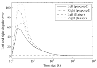
For coupled algorithms,we define the left and right singular error at the k-th update:
| $ \epsilon_L(k)=\|\sigma(k)^{-1}A^{\rm T}{u}(k)-{v}(k)\|, $ | (25) |
| $ \epsilon_R(k)=\|\sigma(k)^{-1}A{v}(k)-{u}(k)\|. $ | (26) |
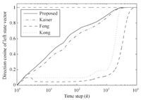
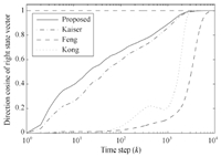
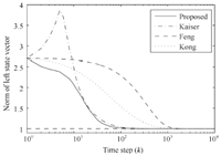
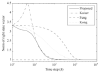
If these two singular errors converge to 0,then the singular value estimate $\sigma(k)$ must approach the true singular value as $k \rightarrow \infty$. In this experiment,the learning rate is chosen as $\gamma = 0.02$ for all rules. The initial value ${u}$(0) and ${v}$(0) are set to be orthogonal to $\bar{{u}}_1$ and $\bar{{v}}_1$. Experiment results are shown in Figs. 1-6.
|
Download:
|
| Fig. 1. Direction cosine between ${u}(k)$ and $\bar{{u}}_1$. | |
|
Download:
|
| Fig. 2. Direction cosine between ${v}(k)$ and $\bar{{v}}_1$. | |
|
Download:
|
| Fig. 3. Norm of left state vector ${u}(k)$. | |
|
Download:
|
| Fig. 4. Norm of left state vector ${v}(k)$. | |
|
Download:
|
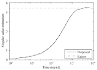
| Fig. 5. Principal singular value estimation, the true principal eigenvalue is indicated by a dashed line. | |
|
Download:
|
| Fig. 6. The left and right singular error. | |
From Figs. 1 and 2,it is observed that all algorithms can effectively extract both of the left and right principal singular vectors of a cross-correlation matrix between two data streams. The coupled algorithms have higher convergence speed than Feng's algorithm. Compared with Kong's algorithm,the coupled algorithms have similar convergence speed in the whole process but higher convergence speed in the beginning steps. In Figs. 3 and 4,we find that all left and right state vectors of all algorithms converge to a unit length,and coupled algorithms have higher convergence speed than noncoupled algorithms. What is more,the principal singular value of the cross-correlation matrix can also be estimated in coupled algorithms,which is actually an advantage of coupled algorithms over noncoupled algorithms. This is very helpful in some engineering applications when singular values estimation is required. Figs. 5 and 6 confirmed the efficiency of principal singular value estimation of coupled algorithms.
In order to demonstrate the estimation accuracy more clearly,we also compute the mean value of the last 100 steps of all aforementioned indices,respectively. The results are shown in Table Ⅰ. We find that the coupled algorithms extract the principal singular vectors more exactly than the noncoupled algorithms.
|
|
Table Ⅰ MEAN VALUES OF THE LAST 100 STEPS OF ALL INDICES |
Here we use the proposed algorithm to extract multiple principal singular component,i.e.,the first 3 PSTs of a cross-covariance matrix,in this experiment. The initial conditions are set to be the same as that in Experiment 1. The method of multiple component extraction is a sequential method,which was introduced in [4]:
| $ A_1(k)=A(k), $ | (27) |
| $ A_i(k)=A_1(k)-\sum^{i-1}_{j=1}{u}_j(k){u}_j^{\rm T}(k)A_1(k){v}_j(k){v}_j^{\rm T}(k)\nonumber\\ =A_{i-1}(k-1)-{u}_{i-1}(k){u}_{i-1}^{\rm T}(k)A_1(k){v}_{i-1}(k){v}_{i-1}^{\rm T}(k),\nonumber\\ \ \ \ \ (i=2,\ldots,n), $ | (28) |
where $A(k)$ is defined in (3) and can be updated as
| $ A(k)=\frac{k-1}{k}A(k-1)+\frac{1}{k} {x}(k){y}^{\rm T}(k). $ | (29) |
By replacing $A$ with $A_i(k)$ instead of $\xi(k)\zeta(k)$ in (15)-(17) at each step,then the i-th triplet (${u}_i, {v}_i,\sigma_i$) can be estimated. In this experiment,we set $\alpha=1$.
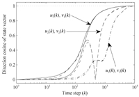
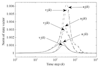
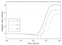
Fig. 7 shows the direction cosine between the first 3 (left and right) principal singular vectors and the true (left and right) singular vectors. Fig. 8 shows the norm of first 3 (left and right) principal singular vectors. And Fig. 9 shows the first 3 principal singular values estimation. Figs. 7-9 confirm the ability of multiple component analysis of proposed algorithm. The results of Experiment 2 confirm the ability of multiple component analysis of proposed algorithm.
|
Download:
|
| Fig. 7. Direction cosine between state vectors (${u}_i(k)$ and ${v}_i(k)$, where $i = 1, 2, 3$) and true singular vectors ($\bar{{u}}_i$ and $\bar{{v}}_i$), respectively. | |
|
Download:
|
| Fig. 8. Norm of all left and right state vectors (${u}_i(k)$ and ${v}_i(k)$, where $i = 1, 2, 3$). | |
|
Download:
|
| Fig. 9. Principal singular values estimation. | |
In this paper,a novel CSVD algorithm is presented by finding the stable stationary point of an NIC via Newton's method. The proposed algorithm can solve the speed-stability problem and thus perform much better than noncoupled algorithms. CSVD algorithms can track the left and right singular vectors and singular value simultaneously,which is very helpful in some engineering applications. The major work in this paper extends the field of CSVD algorithms. Experiment results show that the proposed algorithm performs well.
APPENDIX A APPROXIMATION OF THE INVERSE HESSIANNewton's method requires an inversion on the Hessian (12) in the vicinity of the stationary point,here the PST. The inversion of the Hessian is simplified by a similarity transformation,using the orthogonal matrix
| $ {T}=\left( \begin{array}{ccc} {\bar{U}}&{{0}_{mn}}&{{0}_m}\\ {{0}_{nm}}&{\bar{V}}&{{0}_n}\\ {{0}_m^{\rm T}}&{{0}_n^{\rm T}}&{1} \end{array} \right). $ | (A1) |
Here,$\bar{U} = [\bar{{u}}_1,\ldots,\bar{{u}}_m]$ and $\bar{V} = [\bar{{v}}_1,\ldots,\bar{{v}}_n]$ are matrices which contain all left and right singular vectors in their columns,respectively.
For the computation of the transformed matrix ${H}^\ast = {T}^{\rm T}HT$ we exploit $A^{\rm T}\bar{U} = \bar{V}\bar{S}^{\rm T}$ and $A\bar{V} = \bar{U}\bar{S}$; here $\bar{S}$ is a $m\times n$ matrix whose first $N$ diagonal elements are the singular values arranged in decreasing order,and all remaining elements of $\bar{S}$ are zero. Moreover,in the vicinity of the stationary point $(\bar{{u}}_1,\bar{{v}}_1,\bar{\sigma}_1)$,we can approximate $\bar{{u}}^{\rm T}{u} \approx {e}_m $ and $\bar{{v}}^{\rm T}{v} \approx {e}_n$; here ${e}_m $ and ${e}_n$ are unit vectors of the specified dimensions with a 1 as the first element. We obtain
| $ {H}_0^\ast=\left( \begin{array}{ccc} {-\sigma {I}_m}&{\bar{S}}&{-{e}_m}\\ {\bar{S}^{\rm T}}&{-\sigma {I}_n}&{-{e}_n}\\ {-{e}_m^{\rm T}}&{-{e}_n^{\rm T}}&{0} \end{array} \right). $ | (A2) |
Next,by approximating $\sigma \approx \bar{\sigma}_1$ and by assuming $|\bar{\sigma}_1| \gg |\bar{\sigma}_j|,\forall j = 2,…,M$,the expression $\bar{S}$ can be approximated as $\bar{S} = \sigma\sigma^{-1}\bar{S} \approx \sigma{e}_m{e}_n^{\rm T}$. In this case,(A2) yields
| $ {H}^\ast=\left( \begin{array}{ccc} {-\sigma {I}_m}&{\sigma{e}_m{e}_n^{\rm T}}&{-{e}_m}\\ {\sigma{e}_n{e}_m^{\rm T}}&{-\sigma {I}_n}&{-{e}_n}\\ {-{e}_m^{\rm T}}&{-{e}_n^{\rm T}}&{0} \end{array} \right). $ | (A3) |
As introduced in [21],suppose that an invertible matrix of size $(j+1) \times (j+1)$ is of the form
| $ {R}_{j+1}=\left( \begin{array}{cc} {{R}_j}&{{r}_j}\\ {{r}_j^{\rm T}}&{\rho_j} \end{array} \right), $ | (A4) |
where ${r}_j$ is a vector of size j and $\rho_j$ is a real number. If ${R}_j$ is invertible and ${R}_j^{-1}$ is known,then ${R}_{j+1}^{-1}$ can be determined from
| $ {R}_{j+1}^{-1}=\left( \begin{array}{cc} {{R}_j^{-1}}&{{0}_j}\\ {{0}_j^{\rm T}}&{0} \end{array} \right)+\frac{1}{\beta_j}\left( \begin{array}{cc} {{b}_j{b}_j^{\rm T}}&{{b}_j}\\ {{b}_j^{\rm T}}&{1} \end{array} \right), $ | (A5) |
where
| $ {b}_j=-{R}_j^{-1}{r}_j, $ | (A6) |
| $ \beta_j=\rho_j+{r}_j^{\rm T}{b}_j. $ | (A7) |
Here,it is obvious that ${r}_j=[{e}_m^{\rm T},{e}_n^{\rm T}]^{\rm T}$,$\rho_j=0$ and
| $ {R}_j=\left( \begin{array}{cc} {-\sigma {I}_m}&{\sigma{e}_m{e}_n^{\rm T}}\\ {\sigma{e}_n{e}_m^{\rm T}}&{-\sigma {I}_n}\\ \end{array} \right). $ | (A8) |
Based on the method introduced in [22] and [23],we obtain
| $ {R}_j^{-1}=\left( \begin{array}{cc}\label{Rj_inv} {-\sigma {I}_m}{\sigma{e}_m{e}_n^{\rm T}}\\ {\sigma{e}_n{e}_m^{\rm T}}{-\sigma {I}_n}\\ \end{array} \right)^{-1}\nonumber\\ =-\sigma^{-1}\left( \begin{array}{cc} {({I}_m-{e}_m{e}_m^{\rm T})^{-1}}{{e}_m{e}_n^{\rm T}({I}_n-{e}_n{e}_n^{\rm T})^{-1}}\\ {{e}_n{e}_m^{\rm T}({I}_m-{e}_m{e}_m^{\rm T})^{-1}}{({I}_n-{e}_n{e}_n^{\rm T})^{-1}}\\ \end{array} \right). $ | (A9) |
It is found that ${I}_m-{e}_m{e}_m^{\rm T}$ and ${I}_n-{e}_n{e}_n^{\rm T}$ are singular and thus we add a penalty term $\varepsilon \approx 1$ to (A9),then it yields
| $ {R}_j^{-1}\nonumber\approx\\ -\sigma^{-1}\left( \begin{array}{cc} {({I}_m-\varepsilon{e}_m{e}_m^{\rm T})^{-1}}{{e}_m{e}_n^{\rm T}({I}_n-\varepsilon{e}_n{e}_n^{\rm T})^{-1}}\\ {{e}_n{e}_m^{\rm T}({I}_m-\varepsilon{e}_m{e}_m^{\rm T})^{-1}}{({I}_n-\varepsilon{e}_n{e}_n^{\rm T})^{-1}}\\ \end{array} \right)\nonumber\\ =-\sigma^{-1}\left( \begin{array}{cc} {{I}_m+\eta{e}_m{e}_m^{\rm T}}{(1+\eta){e}_m{e}_n^{\rm T}}\\ {(1+\eta){e}_n{e}_m^{\rm T}}{{I}_n+\eta{e}_n{e}_n^{\rm T}}\\ \end{array} \right), $ | (A10) |
where $\eta=\varepsilon/(1-\varepsilon)$. Thus
| $ {b}_j=-{R}_j^{-1}{r}_j=-2(1+\eta)\sigma^{-1}[{e}_m^{\rm T},{e}_n^{\rm T}]^{\rm T}, $ | (A11) |
| $ \beta_j=\rho_j+{r}_j^{\rm T}{b}_j=4(1+\eta)\sigma^{-1}. $ | (A12) |
Substituting (A10)-(A12) into (A5),it yields
| $ ({H})^{\ast-1}={R}_{j+1}^{-1}\nonumber\approx\\ \left( \begin{array}{ccc} {-\sigma^{-1}({I}_m-{e}_m{e}_m^{\rm T})}{{0}_{mn}}{-\frac{1}{2}{e}_m}\\ {{0}_{nm}}{-\sigma^{-1}({I}_n-{e}_n{e}_n^{\rm T})}{-\frac{1}{2}{e}_n}\\ {-\frac{1}{2}{e}_m^{\rm T}}{-\frac{1}{2}{e}_n^{\rm T}}{\frac{\sigma}{4(1+\eta)}} \end{array} \right). $ | (A13) |
From the inverse transformation ${H}^{-1} = {TH}^{\ast-1}{T}^{\rm T}$ and by approximating $\frac{\sigma}{4(1+\eta)} = \frac{1}{4}\sigma(1-\varepsilon) \approx 0$ ,we get
| $ {H}^{-1}\nonumber\approx\\ \left( \begin{array}{ccc} {-\sigma^{-1}({I}_m-{uu}^{\rm T})}{{0}_{mn}}{-\frac{1}{2}{u}}\\ {{0}_{nm}}{-\sigma^{-1}({I}_n-{vv}^{\rm T})}{-\frac{1}{2}{v}}\\ {-\frac{1}{2}{u}^{\rm T}}{-\frac{1}{2}{v}^{\rm T}}{0} \end{array} \right), $ | (A14) |
where we approximated the unknown singular vectors by $\bar{{u}}_1 \approx {u}$ and $\bar{{v}}_1 \approx {v}$.
APPENDIX B APPROXIMATION ERROR OF INVERSE HESSIAN MATRIXThe approximation error generated by the approximation of the inverse Hessian matrix is defined as
| $ \Delta_{{H}^{-1}}={H}_0^{-1} - {H}^{-1}, $ | (A15) |
where ${H}^{-1}$ is the approximated inverse Hessian that has been calculated in (43); ${H}_0^{-1}$ is the true inverse matrix of Hessian (12) at the stationary point $(\bar{{u}}_1,\bar{{v}}_1,\bar{\sigma}_1)$. The transformed matrix ${H}_0^\ast = {T}^{\rm T}{H}_0{T}$ is shown in (31). In this case, we calculate the inverse of (31) at first,which is
| $ ({H}_0^\ast)^{-1}=\left( \begin{array}{ccc} {{Y}^{\ast}-\sigma^{-1}({I}_m-{e}_m{e}_m^{\rm T})}&{{Z}^{\ast}} &{-\frac{1}{2}{e}_m}\\ {{Z}^{\ast {\rm T}}}& {{X}^{\ast}}&{-\frac{1}{2}{e}_n}\\ {-\frac{1}{2}{e}_m^{\rm T}}&{-\frac{1}{2}{e}_n^{\rm T}}&{0} \end{array} \right), $ | (A16) |
where ${Y}^{\ast}=\sigma^{-2}\bar{S}{X}^{\ast} \bar{S}^{\rm T}$, ${Z}^{\ast}=\frac{1}{2}\sigma^{-1}{e}_m {e}_n^{\rm T}+\sigma^{-1}\bar{S}{X}^{\ast}$ and ${X}^{\ast}=(\sigma^{-1}\bar{S}^{\rm T}\bar{S}-\sigma{I}_n-4\sigma{e}_n{e}_n^{\rm T})^{-1}$. The true inverse Hessian is
| $ {H}_0^{-1}={T}({H}_0^\ast)^{-1}{T}^{\rm T}\nonumber\\ =\left( \begin{array}{ccc} {{Y}-\sigma^{-1}({I}_m-{uu}^{\rm T})}{{Z}} {-\frac{1}{2}{u}}\\ {{Z}^{\rm T}} {{X}}{-\frac{1}{2}{v}}\\ {-\frac{1}{2}{u}^{\rm T}}{-\frac{1}{2}{v}^{\rm T}}{0} \end{array} \right), $ | (A17) |
where ${Y}=\sigma^{-2}A {X} A^{\rm T}$, ${Z}=\frac{1}{2}\sigma^{-1}{uv}^{\rm T}+\sigma^{-1}A {X} $ and
| $ {X}=\bar{V}{X}^{\ast}\bar{V}^{\rm T}\nonumber\\ =\bar{V}(\sigma^{-1}\bar{S}^{\rm T}\bar{S}-\sigma{I}_n-4\sigma{e}_n{e}_n^{\rm T})^{-1} \bar{V}^{\rm T}\nonumber\\ =(\sigma^{-1}A^{\rm T}A-\sigma{I}_n-4\sigma{vv}^{\rm T})^{-1}.\tag{A18} $ | (A18) |
Then,the approximation error matrix is
| $ \Delta_{{H}^{-1}}=\left( \begin{array}{ccc} {{Y}}&{{Z}} &{{0}_m}\\ {{Z}^{\rm T}}& {{X}+\sigma^{-1}({I}_n-{vv}^{\rm T})}&{{0}_n}\\ {{0}_m^{\rm T}}&{{0}_n^{\rm T}}&{0} \end{array} \right). $ | (A19) |
Now we calculate the upper bound of the approximation error. It is found that
| $ \Delta_{{H}^{-1}}={T}\Delta_{({H}^{\ast})^{-1}}{T}^{\rm T}, $ | (A20) |
where
| $ \Delta_{({H}^{\ast})^{-1}}={H}_0^{\ast-1}-{H}^{\ast-1}\nonumber\\ =\left( \begin{array}{ccc} {{Y}^{\ast}}{{Z}^{\ast}} {{0}_m}\\ {({Z}^{\ast})^{\rm T}} {{X}^{\ast}+\sigma^{-1}({I}_n-{e}_n{e}_n^{\rm T})}{{0}_n}\\ {{0}_m^{\rm T}}{{0}_n^{\rm T}}{0} \end{array} \right). $ | (A21) |
It holds that
| $ \|\Delta_{{H}^{-1}}\|_{\text{s}}=\|{T}\|_{\text{s}}\cdot\|\Delta_{{H}^{\ast-1}}\|_{\text{s}}\cdot \|{T}^{\rm T}\|_{\text{s}}, $ | (A22) |
where $\|{T}\|_{\text{s}}$ represents the spectrum norm of matrix $T$. Clearly,it holds that $\|{T}\|_{\text{s}} = \|{T}^{\rm T}\|_{\text{s}} = 1$ and $\|\bar{S}\|_{\text{s}}=\|\bar{S}^{\rm T}\|_{\text{s}}=|\sigma_1|$. Then,we have
| $ \|\Delta_{{H}^{\ast-1}}\|_{\text{s}}\leq\|{Y}^\ast\|_{\text{s}}+\|{Z}^\ast\|_{\text{s}}+\|({Z}^{\ast})^{\rm T}\|_{\text{s}}\nonumber\\ +\|{X}^\ast+\sigma^{-1}({I}_n-{e}_n{e}_n^{\rm T})\|_{\text{s}}. $ | (A23) |
Clearly,we have
| $ \|{Y}^\ast\|_{\text{s}}=\|\sigma^{-2}\bar{S}{X}^{\ast}\bar{S}^{\rm T}\|_{\text{s}}\nonumber\\ \leq|\sigma^{-2}|\cdot \|\bar{S}\|_{\text{s}}\cdot \|{X}^{\ast}\|_{\text{s}}\cdot \|\bar{S}^{\rm T}\|_{\text{s}}=\|{X}^{\ast}\|_{\text{s}}, $ | (A24) |
| $ \|{Z}^{\ast {\rm T}}\|_{\text{s}}=\|{Z}^\ast\|_{\text{s}}=\|\frac{1}{2}\sigma^{-1}{e}_m {e}_n^{\rm T} +\sigma^{-1}\bar{S}{X}^{\ast}\|_{\text{s}}\nonumber\\ \leq\|\frac{1}{2}\sigma^{-1}{e}_m {e}_n^{\rm T}\|_{\text{s}}+\|\sigma^{-1} \bar{S}{X}^{\ast}\|_{\text{s}}\nonumber\\ \leq\frac{1}{2}|\sigma^{-1}|+\|{X}^{\ast}\|_{\text{s}}, $ | (A25) |
and
| $ \|{X}^{\ast}+\sigma^{-1}({I}_n-{e}_n{e}_n^{\rm T})\|_{\text{s}}\nonumber\\ \leq\|{X}^{\ast}\|_{\text{s}}+\|\sigma^{-1}({I}_n-{e}_n{e}_n^{\rm T})\|_{\text{s}}=\|{X}^{\ast}\|_{\text{s}}+|\sigma^{-1}|. $ | (A26) |
From (49) to (55),we conclude that
| $ \|\Delta_{{H}^{-1}}\|_{\text{s}}\leq 4\|{X}^{\ast}\|_{\text{s}}+2|\sigma^{-1}|, $ | (A27) |
where
| $ \|{X}^{\ast}\|_{\text{s}}=\|(\sigma^{-1}\bar{S}^{\rm T}\bar{S}-\sigma{I}_n-4\sigma {e}_n {e}_n^{\rm T})^{-1} \|_{\text{s}}\nonumber\\ =\left\|\left( \begin{array}{cccc} {-4\sigma}{}{}{}\\ {}{\frac{\sigma_2^2}{\sigma}-\sigma}{}{}\\ {}{}{\ddots}{}\\ {}{}{}{\frac{\sigma_n^2}{\sigma}-\sigma} \end{array}\right)^{-1}\right\|_{\text{s}}\nonumber\\ =\left\|\left( \begin{array}{cccc} {-\frac{1}{4}\sigma^{-1}}{}{}{}\\ {}{\frac{\sigma}{\sigma_2^2-\sigma^2}}{}{}\\ {}{}{\ddots}{}\\ {}{}{}{\frac{\sigma}{\sigma_n^2-\sigma^2}} \end{array}\right)\right\|_{\text{s}}\nonumber\\ =\frac{|\sigma|}{\sigma^2-\sigma_2^2} $ | (A28) |
and $\sigma=\bar{\sigma}_1$. Thus,we get
| $ \|\Delta_{{H}^{-1}}\|_{\text{s}}\leq\frac{4|\bar{\sigma}_1|}{\bar{\sigma}_1^2-\bar{\sigma}_2^2}+2|\bar{\sigma}_1^{-1}|. $ | (A29) |
The approximation error of (14) is
| $ \left[\begin{array}{c} {\Delta\dot{{u}}}\\ {\Delta\dot{{v}}}\\ {\Delta\dot{\sigma}} \end{array} \right] = -\Delta_{{H}^{-1}}\nabla p= -\Delta_{{H}^{-1}} \left[ \begin{array}{c} {\frac{\partial p}{\partial {u}}}\\ {\frac{\partial p}{\partial {v}}}\\ {\frac{\partial p}{\partial \sigma}} \end{array} \right]. $ | (A30) |
Since stability analysis shows that the proposed algorithm converges to stationary point $({u}_1,{v}_1,\sigma_1)$ and the approximation error of $\Delta_{{H}^{-1}}$ is bounded,we have
| $ \Delta\dot{{u}}=-{Y}({A}{v}-\sigma{u})-{Z}(A^{\rm T}{u}-\sigma{v})\approx{0}_m, $ | (A31) |
| $ \Delta\dot{{v}}=-{Z}^{\rm T}({A}{v}-\sigma {u})\nonumber\\ -[{X}+\sigma^{-1}({I}_n-{vv}^{\rm T})](A^{\rm T}{u}-\sigma{v})\approx{0}_n, $ | (A32) |
| $ \Delta\dot{\sigma}=0 $ | (A33) |
in the vicinity of stationary point $({u}_1,{v}_1,\sigma_1)$. Thus,the approximation error of (14) is approximate to 0.
| [1] | Kaiser A, Schenck W, Möoller R. Coupled singular value decomposition of a cross-covariance matrix. International Journal of Neural Systems, 2010, 20(4): 293-318 |
| [2] | Cochocki A, Unbehauen R. Neural Networks for Optimization and Signal Processing. New York: John Wiley, 1993. |
| [3] | Yuille A L, Kammen D M, Cohen D S. Quadrature and the development of orientation selective cortical cells by Hebb rules. Biological Cybernetics, 1989, 61(3): 183-194 |
| [4] | Feng D Z, Bao Z, Zhang X D. A cross-associative neural network for SVD of non-squared data matrix in signal processing. IEEE Transactions on Neural Networks, 2001, 12(5): 1215-1221 |
| [5] | Diamantaras K I, Kung S Y. Cross-correlation neural network models. IEEE Transactions on Signal Processing, 1994, 42(11): 3218-3223 |
| [6] | Bunch J R, Nielsen C P. Updating the singular value decomposition. Numerische Mathematik, 1978, 31(2): 111-129 |
| [7] | Comon P, Golub G H. Tracking a few extreme singular values and vectors in signal processing. Proceedings of the IEEE, 1990, 78(8): 1327-1343 |
| [8] | Ferzali W, Proakis J G. Adaptive SVD algorithm for covariance matrix eigenstructure computation. In: Proceedings of the 1990 International Conference on Acoustics, Speech, and Signal Processing. Albuquerque, NM: IEEE, 1990. 2615-2618 |
| [9] | Moonen M, Van Dooren P, Vandewalle J. A singular value decomposition updating algorithm for subspace tracking. SIAM Journal on Matrix Analysis and Applications, 1992, 13(4): 1015-1038 |
| [10] | Helmke U, Moore J B. Singular-value decomposition via gradient and self-equivalent flows. Linear Algebra and Its Applications, 1992, 169: 223-248 |
| [11] | Moore J B, Mahony R E, Helmke U. Numerical gradient algorithms for eigenvalue and singular value calculations. SIAM Journal on Matrix Analysis and Applications, 1994, 15(3): 881-902 |
| [12] | Hori G. A general framework for SVD flows and joint SVD flows. In: Proceedings of the 2003 IEEE International Conference on Acoustics, Speech, and Signal Processing. Hong Kong: IEEE, 2003. II-693-6 |
| [13] | Feng D Z, Bao Z, Shi W X. Cross-correlation neural network models for the smallest singular component of general matrix. Signal Processing, 1998, 64(3): 333-346 |
| [14] | Feng D Z, Zhang X D, Bao Z. A neural network learning for adaptively extracting cross-correlation features between two high-dimensional data streams. IEEE Transactions on Neural Networks, 2004, 15(6): 1541-1554 |
| [15] | Hasan M A. A logarithmic cost function for principal singular component analysis. In: Proceedings of the 2008 IEEE International Conference on Acoustics, Speech, and Signal Processing. Las Vegas, NV: IEEE, 2008. 1933-1936 |
| [16] | Kong X Y, Ma H G, An Q S, Zhang Q. An effective neural learning algorithm for extracting cross-correlation feature between two highdimensional data streams. Neural Processing Letters, 2015, 42(2): 459-477 |
| [17] | Cheng L, Hou Z G, Tan M. A simplified neural network for linear matrix inequality problems. Neural Processing Letters, 2009, 29(3): 213-230 |
| [18] | Cheng L, Hou Z G, Lin Y, Tan M, Zhang W C, Wu F X. Recurrent neural network for non-smooth convex optimization problems with application to the identification of genetic regulatory networks. IEEE Transactions on Neural Networks, 2011, 22(5): 714-726 |
| [19] | Liu Q S, Huang T W, Wang J. One-layer continuous-and discretetime projection neural networks for solving variational inequalities and related optimization problems. IEEE Transactions on Neural Networks and Learning Systems, 2014, 25(7): 1308-1318 |
| [20] | Möoller R, Köonies A. Coupled principal component analysis. IEEE Transactions on Neural Networks, 2004, 15(1): 214-222 |
| [21] | Noble B, Daniel J W. Applied Linear Algebra (Third edition). Englewood Cliffs, NJ: Prentice Hall, 1988. |
| [22] | Hotelling H. Some new methods in matrix calculation. The Annals of Mathematical Statistics, 1943, 14(1): 1-34 |
| [23] | Hotelling H. Further points on matrix calculation and simultaneous equations. The Annals of Mathematical Statistics, 1943, 14(4): 440-441 |
 2016, Vol.3


