 2016, Vol.3


2. Department of Mechanical and Automation Engineering, The Chinese University of Hong Kong, Shatin, New Territories, Hong Kong, China;
3. Department of Computer Science, City University of Hong Kong, Kowloon, Hong Kong, China
The memeristor conceived by [1] is viewed as the fourth circuit element[2]. The memristor and memristor-based circuits have revoked considerable attention since 2008 when its prototype was made by HP Lab[3]. The value of the memristor (i.e.,memristance) depends on the quantity of charge that has passed through the device. Therefore,the memristor can memorize its past dynamic history. Such memory features make the memristor as a promising candidate to simulate biological synapses. As a result,recently,many research has been devoted to investigating memristive neural networks (MNNs),in which the connections between every two neurons are implemented by the memristors instead of the conventional resistors[4, 5].
Some dynamic properties of neural networks,such as stability,passivity have been extensively investigated[6, 7, 8, 9, 10, 11] and recently considered for MNNs,see [12, 13, 14, 15, 16, 17]. Especially,the locality of equilibrium points and the state convergence of MNNs are elaborately discussed in [16] and [17]. It was shown that the model of MNNs can possess more computation and information storage than conventional neural networks,which enlarge the application of neural networks in associative memory and information processing. In addition,the dynamic behaviors of MNNs provide us an important step to understand brain activities.
In 1990,Pecora and Carroll firstly proposed a driving-response law for synchronization of coupled chaotic systems. Since then,synchronization of chaotic systems has been extensively investigated by the researchers from different scientific communities due to its wide applications such as secure communication[18],information processing[19] and pattern recognition[20]. Especially,synchronization of complex dynamical networks has also been extensively studied,see [21, 22, 23, 24, 25, 26, 27, 28, 29, 30, 31, 32] and the references therein. Many static or dynamic control approaches have been proposed for synchronization,including feedback control[33],adaptive control[34],sample-data control[35] and impulsive control[36]. Recently,the synchronization problem has been extended to MNNs[37, 38, 39, 40, 41, 42, 43, 44, 45]. Due to the features of memristor,the MNN can be viewed as a state-dependent switching system. Some novel control laws were designed to synchronize the two MNNs. In [39],a fuzzy model employing parallel distributed compensation (PDC) was proposed and then the periodically intermittent control method was studied in [40]. In [43],a novel control law which consisted of linear feedback and discontinuous feedback was proposed to guarantee synchronization of two MNNs. Then the similar control method was employed to study the synchronization of a class of memristor-based Cohen-Grossberg neural networks with time-varying discrete delays and unbounded distributed delays[41].
As pointed out in [46],in real nervous systems,synaptic transmission is a noisy process brought about by random fluctuations from the release of neurotransmitters and other probabilistic causes. At training recurrent neural network architectures,the model is stochastic owing to the additive presence of process noise and measurement noise,they are assumed to be white noise which makes a digital computer well suited for its implementation[47]. Therefore,the noise is ubiquitous in both nature and man-made neural networks. As so far,there have been many results on the dynamics of conventional neural networks with stochastic noise[48, 49, 50, 51, 52, 53, 54],the synchronization problem of conventional neural networks with additive noise was studied. More recently,exponential synchronization is studied for MNNs in the presence of noise by using impulsive control[55] and discontinuous state feedback control[56].
In this paper,we continue to investigate the master-slave synchronization of MNNs in the presence of additive noise. A stochastic differential equation model is proposed to describe the influence of additive noise on MNNs. By utilizing the stability theory of stochastic differential equations[57],two different control laws are proposed for ascertaining global synchronization in mean square. First,a control law consisting of a time-delay feedback term and a discontinuous feedback term is designed. Sufficient conditions of global synchronization in mean square are derived based on linear matrix inequalities(LMIs). Thereafter,by letting the control gains be dynamical,an adaptive control law consisting of a linear feedback term and a discontinuous feedback term is designed. In this case,the LMI conditions in previous result are removed,which makes the results more practical.
The rest of this paper is organized as follows. In Section Ⅱ,some preliminaries on MNNs with random disturbances are given. In Section Ⅲ,two different control laws are designed and sufficient conditions are derived to ascertain master-slave synchronization in mean square. In Section Ⅳ,two numerical examples are given to substantiate the theoretical results. Concluding remarks are finally drawn in Section Ⅴ.
Ⅱ. PRELIMINARIES AND MODEL FORMULATIONIn this section,preliminary information on memristor and MNNs is given. In addition,we introduce some assumptions,notations,definitions and lemmas.
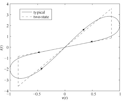
To describe the pinched hysteresis feature (see Fig. 1 of a memristor[1, 2],we utilize the following definition of the memductance[14, 15]:
| $\begin{equation}\label{memrisitor1} W(v(t))=\left\{\begin{array}{cc}W^{\prime}(v(t)),& {\rm D}^-v(t)<0;\\W^{\prime\prime}(v(t)),& {\rm D}^-v(t)>0;\\ W(v(t^-)),&{\rm D}^-v(t)=0,\end{array}\right. \end{equation}$ | (1) |

|
Download:
|
| Fig. 1. The current-voltage characteristic of memristor with a sinusoidal current source. The horizontal coordinate refers to voltage across the memristor while the vertical coordinate refers to the current going through the memristor. The blue solid line and red dash line depict the typical and two-state pinched hysteresis loop, respectively. | |
where $v(t)$ denotes the voltage applied to the memristor,$W(v(t))$ is the memductance of the voltage-controlled memristor,${\rm D}^-v(t)$ means the left Dini-derivation of $v(t)$ in $t$,$W(v(t^-))$ is the left limit of $W(v(t))$ in $t$. $W(v(t^-))$ is either equal to $W^{\prime}(v(t))$ or $W^{\prime\prime}(v(t))$. Obviously,the memductance function may be discontinuous.
As stated in [58],for digital computer applications requiring only two memory states,the memristor needs to exhibit only two sufficiently distinct equilibrium states $R_0$ and $R_1$ where $R_0\gg R_1$,and such that the high-resistance states can be easily switched to the low resistance state,and vice versa,as fast as possible while consuming as little energy as possible. The two-state current-voltage characteristic of this memristor is depicted in Fig. 1. Obviously,it is a special case of (1). Therefore,the memductance of the memristor with this property can be defined as follows:
| $\begin{equation}\label{memrisitor-constant} W(v(t))=\left\{\begin{array}{cc}W^{\prime},& {\rm D}^-v(t)<0;\\W^{\prime\prime},& {\rm D}^-v(t)>0;\\ W(v(t^-)),&{\rm D}^-v(t)=0,\end{array}\right. \end{equation}$ | (2) |
where $W^{\prime}$ and $W^{\prime\prime}$ are constants.
A MNN can be constructed by using memristors to replace resistors in conventional neural networks[4, 5]. In the following,we consider the following dynamical system for recurrent memristive neural networks (RMNN) in the presence of random disturbances[55]:
| $\begin{align}\label{eq:master_system} {\rm d} x(t) = &[-C x(t) + A( x(t) ) f( x(t) ) \notag \\ & + B( x(t) ) f( x(t-\tau(t)) )] {\rm d}t \notag\\ &+ \sigma(t,x(t),x(t-\tau(t))) {\rm d}w(t), \end{align}$ | (3) |
where $x(t) \in {\bf{R}}^n$ is the state of the networks; $f(\cdot)$ corresponds to the activation functions of neurons; $\tau(t)$ is the time-varying delay; $A(x) = [a_{ij}( f_j( x_j(t) ) - x_i(t) )]_{n\times n}$ and $B(x) = [b_{ij}( f_j(x_j(t-\tau(t))) - x_i(t) )]_{n\times n}$ are the feedback memristive connection weight matrix and the delayed feedback memristive connection weight matrix,respectively. The functions $a_{ij}(\cdot)$ and $b_{ij}(\cdot)$ are defined as (2),namely,each connection weight switches between two different values. Here,the values of the functions $a_{ij}(\cdot)$ and $b_{ij}(\cdot)$ are denoted as $\{a_{ij}',a_{ij}''\}$ and $\{b_{ij}',b_{ij}''\}$ respectively. Furthermore,denote $\hat{a}_{ij}=\max\{a_{ij}',a_{ij}''\}$,$\check{a}_{ij} = \min\{a_{ij}',a_{ij}''\}$,$\hat{b}_{ij}=\max\{b_{ij}',b_{ij}''\}$ and $\check{b}_{ij} = \min\{b_{ij}',b_{ij}''\}$. $w(t)=(w_1(t),$ $ w_2(t),$ $\ldots,$ $ w_n(t))$ is a $n$ dimension Brown motion defined on a complete probability space $(\Omega,\mathcal{F,P})$ with a natural filtration $\{\mathcal{F}_t\}_{t\geq 0}$ generated by $\{w(s): 0\leq s \leq \tau\}$,where we associate $\Omega$ with the canonical space generated by $w(t)$,and denote $\mathcal{F}$ the associated $\sigma-$algebra generated by $\{w(t)\}$ with the probability measure $\mathcal{P}$. ${\rm d}w_i(t)$ is the white noise,which is independent of ${\rm d}w_j(t)$ for $j\neq i$. $\sigma: {\bf R}_{+} \times {\bf{R}}^n \times {\bf{R}}^n \to {\bf{R}}^{n \times m}$ is called the noise intensity function matrix. The idea of using memristors to realize MNNs is proposed in [4, 5]. The electronic implementation can be found in [59, 60, 61, 62].
Let ${\pmb L}^2_{\mathcal{F}_0}([-r,0];{\bf{R}}^n)$ denote the family of ${\bf{R}}^n$-valued stochastic process $\{\xi(s),-r\leq s\leq 0\}$,such that $\xi(s)$ is $\mathcal{F}_0$-measurable and $\int_{-r}^0{\rm E}\|\xi(s)\|^2{\rm d}s<\infty$,where ${\rm E}(\cdot)$ is the mathematical expectation.
The initial condition of (3) is $x(t)=\varphi(t),t\in [-r,0]$,where $\varphi\in {\pmb L}^2_{\mathcal{F}_0}([-r,0];{\bf{R}}^n)$. Denote $x(t; \varphi)$ as the solution of (3) with initial value $\varphi$. It means that $x(t; \varphi)$ is continuous and satisfies (3),and $x(s; \varphi) = \varphi(s),s\in [-r ,0]$.
To establish our main results,the following assumptions are necessary throughout this paper.
Assumption 1. Each function $f_i(\cdot):{\bf R}\to {\bf R},i=1,2,\ldots,n,$ is nondecreasing and globally Lipschitz with a constant $l_i>0$,i.e.,
$$ |f_i(u)-f_i(v)|\leq l_i|u-v|,\quad \forall u,v\in {\bf R}.$$Moreover,$|f_i(u)|\leq \gamma_i$ holds for any $u \in {\bf R}$,where $\gamma_i>0$.
Assumption 2. The noise intensity function matrix $\sigma: {\bf R}_{+}\times {\bf{R}}^n\times {\bf{R}}^n \to {\bf{R}}^{n\times n}$ is uniformly Lipschitz continuous in terms of the norm induced by the trace inner product on the matrices
$$ \begin{align*} & \mathrm{trace}[(\sigma( t,u_1,v_1 ) - \sigma( t,u_2,v_2 ) )^{\rm T} \\ &\qquad \times(\sigma( t,u_1,v_1 ) - \sigma( t,u_2,v_2 )] \\ \leq & \|M_1( u_1-u_2 )\|^2 + \|M_2(v_1-v_2)\|^2,\forall u_1,u_2,v_1,v_2\in {\bf{R}}^n, \end{align*}$$where $M_1$ and $M_2$ are known constant matrices with compatible dimensions.
Assumption 3. $\tau(t)$ is a bounded differential function of time $t$,and satisfies
$$\begin{align*} r = \max_{ t\in {\bf R} } \{ \tau(t) \},\quad \dot{ \tau }(t) \leq h < 1, \end{align*}$$where $r$ and $h$ are positive constants.
In a driving-response scheme,there are two identical RMNNs with different initial conditions. One is called the driving RMNN,and the other one is called the response RMNN. Synchronization will occur when the error of the state variables of the two RMNNs approaches 0 in mean square as time elapses. In this paper,RMNN (3) is considered as the master (or driving) system. The slave (or response) system is
| $\begin{align}\label{eq:slave_system} {\rm d} y(t) = &[-C y(t) + A( y(t) ) f( y(t) ) \notag \\ & + B( y(t) ) f( y(t-\tau(t)) ) + u(t)] {\rm d}t \notag\\ &+ \sigma(t,y(t),y(t-\tau(t))) {\rm d}w(t), \end{align}$ | (4) |
where $u(t)\in {\bf{R}}^n$ is the control vector. The initial condition of (4) is $y(t)=\phi(t),t\in [-r,0]$,where $\phi\in {\pmb L}^2_{\mathcal{F}_0}([-r,0];{\bf{R}}^n)$. The aim of this paper is to design a control vector $u(t)$ to let the slave system synchronize with the master system.
Let $e(t)=y(t)-x(t)$,subtracting (3) from (4) yields the error system:
| $\begin{align} {\rm d} e(t)= & [-C e(t) + A( y(t))f(y(t)) -A( x(t) ) f(x(t)) \notag \\ &+ B( y(t) ) f(y(t-\tau(t))) -B( x(t) ) f(x(t-\tau(t)))\notag\\ &+ u(t)] {\rm d}t+ \sigma(t,e(t),e( t-\tau(t) ) ) {\rm d}w(t), \end{align}$ | (5) |
where $ \sigma(t,e(t),e( t-\tau(t) ) ) = \sigma(t,y(t),y( t-\tau(t) ) ) - \sigma(t,x(t),x( t-\tau(t) ) )$. The initial condition of (5) is $ e(t)=\psi(t)=\phi(t)-\varphi(t),t\in [-r,0]$,where $\psi\in {\pmb L}^2_{\mathcal{F}_0}([-r,0];{\bf{R}}^n)$. Then,the synchronization problem of RMNN (3) and (4) is turned to design control vector $u(t)$ such that $e(t)\rightarrow 0$ in mean square as $t\rightarrow +\infty$. Due to the the influence of additive noise,the definition of stability in mean square will be given as follow:
Definition 1. For error system (5) and every $\psi\in {\pmb L}^2_{\mathcal{F}_0}([-r,0];{\bf{R}}^n)$,the trivial solution (equilibrium point) is global asymptotically stable in the mean square if the following holds:
$$ \begin{align*} \lim_{t\to \infty} {\rm E}\|e(t;\psi)\|^2=0. \end{align*}$$Definition 2. Let $C^{2,1}([-r,+\infty)\times {\bf{R}}^n; {\bf{R}}^+) $ denote the family of all nonnegative functions $V(t,x)$ on $[-r,+\infty)\times {\bf{R}}^n$ which are continuous twice differentiable in $x$ and once differentiable in $t$. If $V\in C^{2,1}([-r,+\infty)\times {\bf{R}}^n; {\bf{R}}^+)$,define the weak infinitesimal operator $\mathcal{L}V$ associated with error (5) as
| $\begin{align} &\mathcal{L}V(t,x) = V_t + V_x[-C e(t)\notag \\ &+ A( y(t))f(y(t)) -A( x(t) ) f(x(t)) \notag \\ &+ B( y(t) ) f(y(t-\tau(t))) -B( x(t) )f(x(t-\tau(t)))\notag\\ &+ u(t)]+{\rm trace}[\sigma^{\rm T}V_{xx}\sigma], \end{align}$ | (6) |
where $V_t =\frac{\partial V(t,x)}{\partial t}$,$V_x =\frac{\partial V(t,x)}{\partial x}$,$V_{xx} =(\frac{\partial^2 V(t,x)}{\partial x_i \partial x_j})_{n\times n}$,and $\sigma=\sigma(t,e(t),e( t-\tau(t) ) )$.
Lemma 1[63] . For any vectors $x,y \in {\bf{R}}^n$ and positive definite matrix $Q\in {\bf{R}}^{n\times n}$,the following matrix inequality holds: $2x^{\rm T} y \leq x^{\rm T} Q x + y^{\rm T} Q^{-1} y$.
Ⅲ. MAIN RESULTSIn this section,we shall present two kinds of discontinuous control laws,i.e.,a time-delay feedback control law and an adaptive feedback control law,and then derive the sufficient conditions for assuring that the response RMNN (4) can be globally exponentially synchronized with RMNN (3).
A. A Time-Delay Control Law with Constant Feedback GainsThe control vector $u(t)$ is designed as
| $\begin{align} u(t) = G_1( e(t) ) + G_2( e(t-\tau(t)) ) + G_3 {\rm sign}( e(t) ), \end{align}$ | (7) |
where $G_1$,$G_2$,and $G_3 \in {\bf{R}}^{n\times n}$ are constant gain matrices is to be determined later. Here,$G_3 = {\rm diag}\{g_{31},g_{32},\ldots,g_{3n}\}$ is a diagonal matrix.
Substituting (7) into error system (5),we have
| $\begin{align} {\rm d} e(t) = & [-(C-G_1) e(t) + G_2(e(t-\tau(t))) + G_3{\rm sign}(e(t))\notag \\ & + A( y(t))f(y(t)) -A( x(t) ) f(x(t)) \notag \\ &+ B( y(t) ) f(y(t-\tau(t))) -B( x(t) ) f(x(t-\tau(t)))\notag\\ &+ u(t)] {\rm d}t+ \sigma(t,e(t),e( t-\tau(t) ) ) {\rm d}w(t). \end{align}$ | (8) |
For convenience,we denote $L = {\rm diag}\{l_1,l_2,\ldots,$ $l_n\}$,$Q={\rm diag}\{q_1,$ $q_2,$ $\ldots,$ $q_n\}$ with $q_i=2\sum_{j=1}^n (|a_{ij}'-a_{ij}''|+|b_{ij}'-b_{ij}''|)\gamma_j$,$\tilde{A}=[\tilde{a}_{ij}]_{n\times n}$ with $\tilde{a}_{ij}\in [\check{a}_{ij},\hat{a}_{ij}]$,and $\tilde{B}=[\tilde{b}_{ij}]_{n\times n}$ with $\tilde{b}_{ij}\in [\check{b}_{ij},\hat{b}_{ij}]$. Then,we have following theorem.
Theorem 1. Let Assumptions 1-3 hold. The RMNN (3) and (4) can achieve global asymptotical synchronization in mean square under the control law (7) if there exist a positive real number $\rho$,positive definite diagonal matrices $P = {\rm diag} \{p_1,p_2,\ldots,p_n\}$ and $D = {\rm diag}\{d_1,d_2,\ldots,d_n\}$,and positive definite matrices $H = [h_{ij}]_{n \times n}$,$R = [r_{ij}]_{n \times n}$,such that
| $N=\left[\begin{matrix} {{\Pi }_{1}} & P{{G}_{2}} & P\tilde{A}+LD & P\tilde{B} \\ * & {{\Pi }_{2}} & 0 & 0 \\ * & * & H-2D & 0 \\ * & * & * & -(1-h)H \\ \end{matrix} \right]<0,$ | (9) |
| $\text{G }\!\!\_\!\!\text{ 3+Q }<\text{0,}$ | (10) |
and
| $\begin{align} P < \rho I \label{eq:thm1-condition3}, \end{align}$ | (11) |
where $\Pi_1 = P(-C+G_1)+(-C+G_1)^{\rm T} P +R +\rho M_1^{\rm T} M_1$ and $\Pi_2 = \rho M_2^{\rm T} M_2-(1-h)R$.
Proof.Consider the following Lyapunov functional:
| $ \begin{align}\label{eq:definition-v} V(t) = \sum_{i=1}^3 V_i(t), \end{align}$ | (12) |
where
| ${{V}_{1}}(t)\text{ }={{e}^{\text{T}}}(t)Pe(t),$ | (13) |
| ${{V}_{2}}(t)=\int_{t-\tau (t)}^{t}{{{e}^{\text{T}}}}(s)Re(s)\text{d}s,$ | (14) |
| ${{V}_{3}}(t)=\int_{t-\tau (t)}^{t}{{{g}^{\text{T}}}}(e(s))Hg(e(s))\text{d}s,$ | (15) |
and P,R and H are given matrices.
From Definition 2,the weak infinitesimal operator $\mathcal{L}$ of the stochastic process $\{x_t = x(t+s),t\geq 0,-r\leq s\leq 0\}$ is operated at $V_1(t)$,$V_2(t)$ and $V_3(t)$ along the trajectory of system (8) under the control law (7):
| $ \begin{align} &\mathcal{L} V_1(t)\notag \\ =& 2 e^{\rm T}(t) P [-(C-G_1) e(t) + G_2(e(t-\tau(t)))\notag \\ & + G_3{\rm sign}(e(t))+ A( y(t))f(y(t)) -A( x(t) ) f(x(t)) \notag \\ &+ B( y(t) ) f(y(t-\tau(t))) -B( x(t) ) f(x(t-\tau(t)))\notag\\ &+ u(t)]+ \mathrm{trace} [\sigma^{\rm T}(t,e(t),e( t-\tau(t) ) ) P \notag \\ &\times \sigma(t,e(t),e( t-\tau(t) ) )]\notag \\ =& 2 e^{\rm T}(t) P [(-C+G_1)e(t) + G_2 e(t-\tau(t)) \notag \\ & + G_3 {\rm sign}(e(t)) + \tilde{A} g( e(t) ) + \tilde{B} g( e(t-\tau(t) ) )\notag \\ & + (A( y(t) ) - \tilde{A}) f(y(t)) + (\tilde{A}-A( x(t) ) ) f(x(t)) \notag \\ & + (B( y(t) ) - \tilde{B}) f(y(t-\tau(t)))\notag \\ & + (\tilde{B}-B( x(t) ) ) f(x(t-\tau(t)))]\notag \\ & + \mathrm{trace} [\sigma^{\rm T}(t,e(t),e( t-\tau(t) ) ) P \notag \\ & \times\sigma(t,e(t),e( t-\tau(t) ) )],\label{eq:thm1-LV1} \end{align}$ | (16) |
| $ \begin{align} \mathcal{L}V_2(t) = & e^{\rm T}(t) R e(t) \notag \\ &- (1-\dot{\tau}(t)) e^{\rm T}(t-\tau(t)) R e(t-\tau(t)),\label{eq:thm1-LV2} \end{align}$ | (17) |
and
| $\begin{align} \mathcal{L}V_3(t) = & g^{\rm T}(t) H g(t) - (1-\dot{\tau}(t)) \notag \\ & \times g^{\rm T}(e(t-\tau(t))) H g(e(t-\tau(t))). \label{eq:thm1-LV3} \end{align}$ | (18) |
Since the activation function $f_i(\cdot)$ is bounded,then we have
| $ \begin{align} & 2e^{\rm T}(t)P(A(y(t))-\tilde{A})f(y(t)) \notag \\ &= 2 \sum_{i=1}^n\sum_{j=1}^n e_i(t)p_i(a_{ij}(y(t))-\tilde{a}_{ij})f_j(y_j(t)) \notag \\ &\leq 2\sum_{i=1}^n\left(\sum_{j=1}^n p_i|a_{ij}'-a_{ij}''|\gamma_j\right)|e_i(t)|. \label{eq:thm1-ePAf1} \end{align}$ | (19) |
Similarly,we can also obtain that
| $ \begin{align} & 2e^{\rm T}(t)P(\tilde{A}-A(x(t)))f(x(t)) \notag \\ &\leq 2\sum_{i=1}^n\left(\sum_{j=1}^n p_i|a_{ij}'-a_{ij}''|\gamma_j\right)|e_i(t)|,\label{eq:thm1-ePAf2} \end{align}$ | (20) |
| $ \begin{align} & 2e^{\rm T}(t)P(B(y(t))-\tilde{B})f(y(t-\tau(t))) \notag \\ &\leq 2\sum_{i=1}^n\left(\sum_{j=1}^n p_i|b_{ij}'-b_{ij}''|\gamma_j\right)|e_i(t)|,\label{eq:thm1-ePBf1} \end{align}$ | (21) |
and
| $ \begin{align} & 2e^{\rm T}(t)P(\tilde{B}-B(x(t)))f(x(t-\tau(t))) \notag \\ &\leq 2\sum_{i=1}^n\left(\sum_{j=1}^n p_i|b_{ij}'-b_{ij}''|\gamma_j\right)|e_i(t)|. \label{eq:thm1-ePBf2} \end{align}$ | (22) |
In addition,we have that
| $ \begin{align} &2e^{\rm T}(t)PG_3 {\rm sign}(e(t)) =2 \sum_{i=1}^n p_i g_{3i} |e_i(t)|. \label{eq:thm1-e-sign} \end{align}$ | (23) |
By Assumption 2 and condition (11),we have
| $ \begin{align}\label{eq:thm1-trace} &\mathrm{trace}[\sigma^{\rm T}(t,e(t),e( t-\tau(t) ) ) P\sigma(t,e(t),e( t-\tau(t) ) )] \notag \\ &\leq \rho \mathrm{trace}[\sigma^{\rm T}(t,e(t),e( t-\tau(t) ) ) \sigma(t,e(t),e( t-\tau(t) ) )] \notag \\ &\leq \rho [e^{\rm T}(t)M_1^{\rm T} M_1 e(t) \notag \\ & \quad + e^{\rm T}(t-\tau(t)) M_2^{\rm T} M_2 e(t-\tau(t))]. \end{align}$ | (24) |
From Assumption 1,it is obvious that
$$ \begin{align*} g^{\rm T}(t) DL e(t) & = \sum_{i=1}^n g_i(t) d_i l_i e_i(t) \notag \\ &\geq \sum_{i=1}^n d_i g_i^2(t) = g^{\rm T}(t) D g(t), \end{align*}$$which implies that
| $\begin{align} \label{eq:thm1-gDKe} g^{\rm T}(t) DL e(t) - g^{\rm T}(t) D g(t) \geq 0. \end{align}$ | (25) |
Let $\eta=[e^{\rm T}(t),e^{\rm T}(t-\tau(t)),g^{\rm T}(e(t)),g^{\rm T}(e(t-\tau(t)))]^{\rm T}$ and combining (9)-(10) and (16)-(25),we have
| $ \begin{align} \label{eq:thm1-lvf} \mathcal{L}V(t) & \leq \sum_{i=1}^3\mathcal{L}V_i(t) + g^{\rm T}(t) DL e(t) - g^{\rm T}(t) D g(t) \notag \\ &\leq \eta^{\rm T} N \eta + 2P(G_3+Q)|e(t)|\leq 0. \end{align}$ | (26) |
From (26) and It ${\rm{\hat o}}$ formula[57],it is obvious to see that
| $\begin{equation} {\rm E}V(t)-{\rm E}V(0)={\rm E}\int_0^t\mathcal{L}V(s){\rm d}s. \end{equation}$ | (27) |
Based on (12),there exists a positive constant $\lambda$ such that
| $\begin{align} \lambda{\rm E}\|e(t)\|^2&\leq {\rm E}V(t)\leq {\rm E}V(0)+{\rm E}\int_0^t\mathcal{L}V(s){\rm d}s \notag \\ &\leq {\rm E}V(0)+\lambda_{\max}{\rm E}\int_0^t\|e(s)\|^2{\rm d}s. \end{align}$ | (28) |
therefore,from (28) and the discussion in [57],we know that the equilibrium of the error system (8) is globally asymptotically stable in mean square.
Remark 1. It is worth noting that the analysis technique in [32, 41] ignored neuronal excitatory and inhibitory effects. In contrast,in Theorem 1,if $G_1,G_2$ and $G_3$ are given,the synchronization conditions are derived in the form of LMIs with a consideration of the neuronal excitatory and inhibitory effects. There are two advantages: first,there is no need to tune any parameters or matrices to derive global synchronization criteria; second,it can be efficiently verified via solving LMIs numerically.
Remark 2. In Theorem 1,we adopt the following decomposition technique:
| $\begin{align}\label{decom1} &A( y(t))f(y(t)) -A( x(t) )f(x(t))\notag \\ =&\tilde{A} g( e(t) ) + (A( y(t) ) - \tilde{A}) f(y(t)) \notag \\ & +(\tilde{A}-A( x(t) ) ) f(x(t)), \end{align}$ | (29) |
and
| $\begin{align}\label{decom2} &B( y(t) ) f(y(t-\tau(t))) -B( x(t) )f(x(t-\tau(t)))\notag\\ =&\tilde{B} g( e(t-\tau(t) ) ) + (B( y(t) ) - \tilde{B}) f(y(t-\tau(t)))\notag\\ & + (\tilde{B}-B( x(t) ) ) f(x(t-\tau(t))). \end{align}$ | (30) |
The results here suggest that it should be worthwhile considering previous results on the synchronization of memristive neural network models by using this decomposition technique.
Remark 3. As MNNs are state-dependent switching systems,the driving system and response system are nonidentical when they have different states. The proof of Theorem 1 shows that the discontinuous term in the control law is used to offset the anti-synchronizing effect arisen by the difference between two RMNNs. Furthermore,the discontinuous feedback control can attenuate the disturbance.
Remark 4. Since the control law (7) is discontinuous,the chattering will occur[64]. In order to eliminate the chattering,(7) can be modified as
$$ u(t) = G_1( e(t) ) + G_2( e(t-\tau(t)) ) + G_3 \frac{e(t)}{|e(t)|+\varepsilon}, $$where
$$ \frac{e(t)}{|e(t)|+\varepsilon}=(\frac{e_1(t)}{|e_1(t)|+\varepsilon_1},\ldots,\frac{e_1(t)}{|e_1(t)|+\varepsilon_1})^{\rm T}, $$and $\varepsilon_i$ is a sufficiently small positive constant for $i=1,2,\ldots,n$.
Let $P=I_n$ in Theorem 1,we have the following corollary:
Corollary 1. Let Assumptions 1-3 hold. The RMNN (3) and (4) can achieve global asymptotical synchronization in mean square under the control law (7) if there exist a positive definite diagonal matrices $D = {\rm diag} \{d_1,d_2,\ldots,d_n\}$,and positive definite matrices $H = [h_{ij}]_{n \times n}$,$R = [r_{ij}]_{n \times n}$,such that
| $ \begin{align} N = \left[\begin{array}{cccc} \Pi_1 & G_2 & \tilde{A}+LD & \tilde{B} \\ \ast & \Pi_2 & 0 & 0 \\ \ast & \ast & H-2D & 0 \\ \ast & \ast & \ast & -(1-h)H \end{array}\right]& <0. \end{align}$ | (31) |
and
| $ \begin{align} G_3+Q & <0. \end{align}$ | (32) |
where $\Pi_1 = (-C+G_1)+(-C+G_1)^{\rm T} +R +M_1^{\rm T} M_1$ and $\Pi_2 = M_2^{\rm T} M_2-(1-h)R$.
In order to show the design of estimate gain matrix $G_1$,$G_2$ and $G_3$,a simple transformation is made to derive the following corollary:
Corollary 2. Let Assumptions 1-3 hold. The RMNN (3) and (4) can achieve global asymptotically synchronization in mean square under the control law (7) if there exist a positive real number $\rho$,positive definite diagonal matrices $P = {\rm diag} \{p_1,p_2,\ldots,p_n\}$ and $D = {\rm diag} \{d_1,d_2,\ldots,d_n\}$,and positive definite matrices $H \in {\bf{R}}^{n \times n}$,$R \in {\bf{R}}^{n \times n}$,and matrices $G_1'\in {\bf{R}}^{n \times n}$,$G_2'\in {\bf{R}}^{n \times n}$ and diagonal matrix $G_3'\in {\bf{R}}^{n \times n}$ such that
| $\begin{array}{*{35}{l}} N=\left[\begin{matrix} {{\Pi }_{1}} & {{G}_{{{2}'}}} & P\tilde{A}+LD & P\tilde{B} \\ * & {{\Pi }_{2}} & 0 & 0 \\ * & * & H-2D & 0 \\ * & * & * & -(1-h)H \\ \end{matrix} \right] & <0,\\ \\ \end{array}$ | (33) |
| ${{G}_{{{3}'}}}+Q\text{ }<\text{0,}$ | (34) |
and
| $ \begin{align} P < \rho I \label{eq:cor1-condition3}, \end{align}$ | (35) |
where $\Pi_1 = -2PC+G_1'+G_1'^{\rm T} +R +\rho M_1^{\rm T} M_1$ and $\Pi_2 = \rho M_2^{\rm T} M_2-(1-h)R$. Moreover,$G_1 = P^{-1}G_1'$,$G_2 = P^{-1}G_2'$,and $G_3 = G_3'$.
Proof. It can be directly verified by letting $G_1 = P^{-1}G_1'$,$G_2 = P^{-1}G_2'$,and $G_3 = G_3'$ in Theorem 1.
Remark 5. Note that,if we set $G_2'={0}$,namely,the time-delay feedback is not utilized,the control law (7) obtained here is consistent with that in [56] and can still synchronize the two MNNs with random disturbances in the sense of mean square. However,the time-delay feedback can reduce the upper bound of the control gain,which will be illustrated in simulation results. Moreover,the time delay is ubiquitous in nature,hence such time-delay feedback will be more meaningful in practice.
Next,we consider the following driving-response pair of MNNs without random disturbances:
| $\begin{align}\label{eq:master_system1} \frac{ {\rm d} x(t)}{{\rm d}t} = &-C x(t) + A( x(t) ) f( x(t) ) \notag \\ & + B( x(t) ) f( x(t-\tau(t)) ), \end{align}$ | (36) |
and
| $\begin{align}\label{eq:slave_system1} \frac{{\rm d} y(t)}{{\rm d}t } = &-C y(t) + A( y(t) ) f( y(t) ) \notag \\ & + B( y(t) ) f( y(t-\tau(t)) ) + u(t). \end{align}$ | (37) |
Based on Theorem 1,we have the following corollaries:
Corollary 3. Let Assumptions 1 and 3 hold. The MNNs (36) and (37) can achieve global asymptotical synchronization under the control law (7) if there exist positive definite diagonal matrices $P = {\rm diag} \{p_1,p_2,\ldots,p_n\}$ and $D = {\rm diag} \{d_1,d_2,\ldots,d_n\}$,and positive definite matrices $H = [h_{ij}]_{n \times n}$,$R = [r_{ij}]_{n \times n}$,such that
| $ \begin{align} N = \left[\begin{array}{cccc} \Pi_1 & PG_2 & P\tilde{A}+LD & P\tilde{B} \\ \ast & -(1-h)R & 0 & 0 \\ \ast & \ast & H-2D & 0 \\ \ast & \ast & \ast & -(1-h)H \end{array}\right]& <0 \end{align}$ | (38) |
and
| $ \begin{equation} G_3+Q <0, \end{equation}$ | (39) |
where $\Pi_1 = P(-C+G_1)+(-C+G_1)^{\rm T} P +R$.
Corollary 4. Assume that Assumption 1 hold and let $G_1={\rm diag}\{g_{11},\ldots,g_{1n}\}$ and $G_2=0$ in (7). The MNNs (36) and (37) can achieve global exponential synchronization under the control law (7) if there exist positive $r_i(i=1,2,\ldots,n)$ such that
| $ \begin{equation} g_{1i}>-c_i+\sum_{j=1}^{n}\frac{r_j}{r_i}l_i(|\tilde{a}_{ji}|+|\tilde{b}_{ji}|) \end{equation}$ | (40) |
and
| $\begin{equation}\label{condition2} g_{3i}\geq 2\sum_{j=1}^{n}[|a_{ij}^{\prime}-a_{ij}^{\prime\prime}|+|b_{ij}^{\prime}-b_{ij}^{\prime\prime}|]\gamma_j. \end{equation}$ | (41) |
Proof. Consider a functional defined by
| $\begin{align}\label{lyapnov1} V(t,e_t)=&{\rm e}^{\delta t}\sum_{i=1}^nr_i|e_{i}(t)|+\sum_{i=1}^{n}\sum_{j=1}^{n}r_{j}|\tilde{b}_{ji}|\notag\\ &\times\int_{t-\tau_{i}}^{t}|g_i(e_i(s))|{\rm e}^{\delta(s+\tau_{i})}{\rm d}s. \end{align}$ | (42) |
Then,as Remark 2 states,using the decomposition technique in Theorem 1 and following the line of the proof of Theorem 1 in [43],the conclusion of the corollary can be easily obtained.
Remark 6. As we know,there exist many results on the master-slave synchronization of MNNs without additive noise,such as [37, 38, 39, 41, 43]. Without the discontinuous control law,only weak synchronization (or bounded synchronization) results,but not complete synchronization results can be obtained in [37, 38, 39]. Compare Corollary 4 with the corresponding results in [41, 43],if the models in [41, 43] are changed into (36) and (37),then (40) is less conservative than (7) and (19) in [41, 43],respectively,this is because for $i,j=1,2,\ldots,n$,
$$ |\tilde{a}_{ij}|\leq \max\{|a^{'}_{ij}|,|a^{''}_{ij}|\}\ \ {\rm and}\ \ |\tilde{b}_{ij}|\leq \max\{|b^{'}_{ij}|,|b^{''}|_{ij}\}. $$If we choose $\tilde{A}=A(x(t))$ or $A(y(t))$,and $\tilde{B}=B(x(t-\tau(t)))$ or $B(y(t-\tau(t)))$ in the decomposition (29) and (30),respectively,we can obtain the same results as that in [41, 43].
B. A Control Law with Adaptive Feedback GainsThe control vector $u(t)$ is designed as follows:
| $\begin{align} u(t) = G_1(t)e(t) + G_3(t) {\rm sign}(e(t)), \end{align}$ | (43) |
where $G_1(t) = {\rm diag}\{g_{11(t)},g_{12}(t),\ldots,g_{1n}(t)\}$ and $G_3(t) = {\rm diag}\{g_{31(t)},g_{32}(t),\ldots,g_{3n}(t)\}$ are time-varying control gain satisfying the following adaptive law:
$$\begin{align*} \dot{g}_{1i}(t) & = -\alpha_i e^2_i(t) \end{align*}$$and
$$\begin{align*} \dot{g}_{3i}(t) & = -\beta_i |e_i(t)|, \end{align*}$$where $\alpha_i,\beta_i>0$ are proper constants,$i=1,2,\ldots,n$.
Theorem 2. Let Assumptions 1-3 hold. The RMNN (3) and (4) can achieve global asymptotically synchronization in mean square under the control law (43).
Proof. Consider the following Lyapunov functional:
| $ \begin{align} V(t) = \sum_{k=1}^3 V_k(t), \end{align}$ | (44) |
where
| ${{V}_{1}}(t)=\frac{1}{2}{{e}^{\text{T}}}(t)e(t),$ | (45) |
| ${{V}_{2}}(t)=\int_{t-\tau (t)}^{t}{{{e}^{\text{T}}}}(s)Re(s)\text{d}s,$ | (46) |
and
| $ \begin{align} V_3(t) & = \sum_{i=1}^n \left(\frac{(g_{1i}(t)+\xi_i)^2}{2\alpha_i}+\frac{(g_{3i}(t)+\phi_i)^2}{2\beta_i}\right), \end{align}$ | (47) |
where $R\in {\bf{R}}^{n\times n}$ is positive definite matrix,and $\xi_i>0$ and $\phi_i>0$ ($i=1,$ $2,$ $\ldots,$ $ n$) are constants to be determined later.
From Definition 2,the weak infinitesimal operator $\mathcal{L}$ of the stochastic process $\{x_t = x(t+s),t\geq 0,-r\leq s\leq 0\}$ is operated at $V_1(t)$,$V_2(t)$ and $V_3(t)$ along the trajectory of system (8) under the control law (43):
| $ \begin{align} \mathcal{L} V_1(t) =& e^{\rm T}(t) [(-C+G_1(t))e(t) + G_3(t) {\rm sign}(e(t)) \\ & + \tilde{A} g( e(t) ) + \tilde{B} g( e(t-\tau(t) ) ) \\ & + (A( y(t) ) - \tilde{A}) f(y(t)) + (\tilde{A}-A( x(t) ) ) f(x(t)) \\ & + (B( y(t) ) - \tilde{B}) f(y(t-\tau(t))) \\ & + (\tilde{B}-B( x(t) ) ) f(x(t-\tau(t)))] \\ & + \mathrm{trace} [\sigma^{\rm T}(t,e(t),e( t-\tau(t) ) ) \\ & \times\sigma(t,e(t),e( t-\tau(t) ) )],\label{eq:thm2-LV1} \\\end{align}$ | (48) |
| $ \begin{align}\mathcal{L}V_2(t) = & e^{\rm T}(t) R e(t) \\ &- (1-\dot{\tau}(t)) e^{\rm T}(t-\tau(t)) R e(t-\tau(t)),\label{eq:thm2-LV2} % \mathcal{L}V_3(t) = & g^{\rm T}(t) H g(t) - (1-\dot{\tau}(t)) \\ % & \cdot g^{\rm T}(e(t-\tau(t))) H g(e(t-\tau(t))). \label{eq:thm2-LV3} \end{align}$ | (49) |
and
| $ \begin{align} \mathcal{L}V_3(t) = & -e^{\rm T}(t) G_1(t) e(t) - \sum_{i=1}^n \xi_i e_i(t)^2 \notag \\ &- G_3(t) |e(t)| - \sum_{i=1}^n \phi_i |e_i(t)|. \label{eq:thm2-LV4} \end{align}$ | (50) |
By Lemma 1,and taking $Q$ as the corresponding identity matrix,we have
$$ \begin{align*} e^{\rm T}(t)\tilde{A}g(e(t))\leq \frac{1}{2}e^{\rm T}(t)\tilde{A}\tilde{A}^{\rm T} e(t)+ \frac{1}{2}g^{\rm T}(e(t))g(e(t)) \end{align*}$$and
$$ \begin{align*} &e^{\rm T}(t)\tilde{B}g(e(t-\tau(t))) \notag \\ & \leq\frac{1}{2}e^{\rm T}(t)\tilde{B}\tilde{B}^{\rm T} e(t)+ \frac{1}{2} g^{\rm T}(e(t-\tau(t))) g(e(t-\tau(t))). \end{align*}$$Recalling Assumption 1,we have:
$$\begin{align*} |g_i(e_i(t))| & \leq l_i|e_i(t)| \end{align*}$$and
$$\begin{align*} |g_i(e_i(t-\tau(t)))| & \leq l_i |e(t-\tau(t))|, \end{align*}$$hold for any $ i = 1,2,\ldots,n$. Then we can obtain that
| $\begin{align} g^{\rm T}(e(t))g(e(t)) &= \sum_{i=1}^n g_i^2(e_i(t)) \notag \\ & \leq\sum_{i=1}^n l_i^2 e_i^2(t) = e^{\rm T}(t) L^2 e(t) \end{align}$ | (51) |
and
| $\begin{align} &g^{\rm T}(e(t-\tau(t)))g(e(t-\tau(t))) \notag \\ &\leq e^{\rm T}(t-\tau(t)) L^2 e(t-\tau(t)). \end{align}$ | (52) |
Hence,we have
| $\begin{align} e^{\rm T}(t)\tilde{A}g(e(t)) \leq e^{\rm T}(t)\frac{\tilde{A}\tilde{A}^{\rm T}+L^2}{2}e(t) \label{eq:thm2-eAg} \end{align}$ | (53) |
and
| $\begin{align} & e^{\rm T}(t-\tau(t))\tilde{B}g(e(t-\tau(t))) \notag \\ &\leq e^{\rm T}(t-\tau(t))\frac{\tilde{B}\tilde{B}^{\rm T}+L^2}{2}e(t-\tau(t)). \label{eq:thm2-eBg} \end{align}$ | (54) |
Next,by the similar discussion as (19)-(25) in Theorem 1,and then combining (48)-(50),(53) and (54),we have
| $ \begin{align} \mathcal{L}V(t)&\leq e^{\rm T}(t)\Bigg(-C+R+M_1^{\rm T}M_1 +\frac{\tilde{A}\tilde{A}^{\rm T} + \tilde{B}\tilde{B}^{\rm T}}{2} \notag \\ &+ L^2 -{\xi}\Bigg)e(t) +(Q-{\phi}) |e(t)|, \end{align}$ | (55) |
where ${\xi}={\rm diag}\{\xi_1,$ $ \xi_2,$ $ \ldots,$ $\xi_n\}$ and ${\phi}={\rm diag}\{\phi_1,$ $ \phi_2,$ $ \ldots,$ $ \phi_n\}$. It is easy to find that,$\xi_i$ and $\phi_i$ can be chosen large enough such that
$$\begin{align*} -C+R+M_1^{\rm T}M_1 +\frac{\tilde{A}\tilde{A}^{\rm T} + \tilde{B}\tilde{B}^{\rm T}}{2} + L^2 -{\xi} & \leq 0 \end{align*}$$and
$$ \begin{align*} Q-{\phi} & \leq 0, \end{align*}$$then $\mathcal{L}V(t) \leq 0$. Therefore,similarly to the discussion in Theorem 1,we know that the equilibrium of the error system (5) under the control law (43) is globally asymptotically stable in mean square.
Remark 7. By comparing Theorem 1 and Theorem 2,it can be seen that the information of the parameters on both MNNs and additive noise are not required in advance. Hence,this method can also deal with uncertain disturbances.
Ⅳ. SIMULATION RESULTSIn this section,we elaborate on two numerical examples to substantiate the theoretical results.
Example 1. Consider the following two-neuron memristive cellular neural network with time delay and additive noise:
| $\begin{align}\label{eq:exm1-model} {\rm d}x=&[-x(t)+A(x)f(x(t))+B(x)f(x(t-\tau))]{\rm d}t \notag\\ & +\sigma(t,x(t),x(t-\tau)){\rm d}w, \end{align}$ | (56) |
where $x(t)=(x_1(t),x_2(t))^{\rm T}\in {\bf{R}}^2$,$C=I_2$,$\tau=0.85$,$f(x)=(f_1(x_1),f_2(x_2))^{\rm T}$ with $f_i(x_i)=(|x_i+1|-|x_i-1|)/2$ $(i=1,2)$. The weight matrices $A$ and $B$ have the following forms:
$$\begin{align*} A=\left[\begin{array}{cc} a_{11}(x) & 20 \\ 0.1 & a_{22}(x) \end{array} \right]\; {\rm and}\ \ B=\left[\begin{array}{cc} b_{11}(x) & 0.1 \\ 0.1 & b_{22}(x) \end{array} \right], \end{align*}$$where the value of $a_{ii}(\cdot)$ and $b_{ii}(\cdot)$ depend on the sign of left Dini-derivation of $f_{i}(x_i(t))-x_i(t)$ and $f_{i}(x_i(t-\tau))-x_i(t),i=1,2$,respectively. Denote $f_{ii}(t)=f_{i}(x_i(t))-x_i(t)$ and $f_{ii}(t-\tau)=f_{i}(x_i(t-\tau))-x_i(t)$. $a_{ii}$ and $b_{ii}$ are given by
$$\begin{align*} a_{11}(t)&=\left\{\begin{array}{ll} 1.7854,& {\rm D}^-f_{11}(t)<0;\\ 2.0472,& {\rm D}^-f_{11}(t)>0;\\ a_{11}(t^-),&{\rm D}^-f_{11}(t)=0, \end{array}\right.\\ a_{22}(t)&=\left\{\begin{array}{ll} 1.5236,& {\rm D}^-f_{22}(t)<0;\\ 1.6283,& {\rm D}^-f_{22}(t)>0;\\ a_{22}(t^-),& {\rm D}^-f_{22}(t)=0, \end{array}\right.\\ b_{11}(t)&=\left\{\begin{array}{ll} -2.2214,& {\rm D}^-f_{11}(t-0.85)<0;\\ -1.3329,& {\rm D}^-f_{11}(t-0.85)>0;\\ b_{11}(t^-),& {\rm D}^-f_{11}(t-0.85)=0, \end{array}\right.\\ b_{22}(t)&=\left\{\begin{array}{ll} -1.9252,& {\rm D}^-f_{22}(t-0.85)<0;\\ -1.6661,& {\rm D}^-f_{22}(t-0.85)>0;\\ b_{22}(t^-),& {\rm D}^-f_{22}(t-0.85)=0 \end{array}\right. \end{align*}$$and $\sigma(t,x(t),x(t-\tau))$ is given by
$$\begin{align*} \sigma(t,x(t),x(t-\tau)) = \left[\begin{array}{cc} \sin(x_1(t)) & 0 \\ 0 & 2\cos(x_2(t-0.85)) \end{array}\right]. \end{align*}$$The controlled response system is described by
| $\begin{align}\label{eq:exm12-model} {\rm d}y=&[-y(t)+A(y)f(y(t))+B(y)f(y(t-\tau))\notag\\ &+u(t)]{\rm d}t + \sigma(t,y(t),y(t-\tau)){\rm d}w, \end{align}$ | (57) |
where $u(t)$ is defined in (7).
Obviously,the activation functions $f_i(\cdot)(i=1,2)$ satisfy Assumption 1 with $l_1=l_2=1$ and $\gamma_1=\gamma_2=1$. In addition,we have
| $\begin{align} M_1 = \left[\begin{array}{cc} 1 & 0\\ 0 & 1 \end{array}\right] \quad {\rm and}\quad M_2 = \left[\begin{array}{cc} 2 & 0\\ 0 & 2 \end{array}\right]. \end{align}$ | (58) |
The controller gains are given as
$$\begin{align*} G_1 = \left[\begin{array}{cc} -8 & 0\\ 0 & -8 \end{array}\right]&,\quad G_2 = \left[\begin{array}{cc} -1 & 0\\ 0 & -1 \end{array}\right],\\ G_3 = \left[\begin{array}{cc} -3 & 0\\ 0 & -1 \end{array}\right]&. \end{align*}$$next,we proceed to verify the conditions in theorem 1. according to the definition of $q$,we have
$$\begin{align*} Q = \left[\begin{array}{cc} 2.3006 & 0\\ 0 & 0.7276 \end{array}\right]. \end{align*}$$Thus,we can obtain that $Q+G_3<0$. Then,we solve LMI (9) and the corresponding matrices are given below:
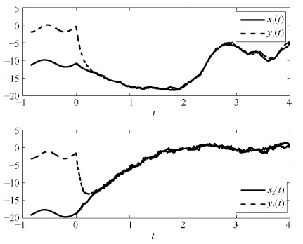
$$\begin{align*} P &= \left[\begin{array}{rr} 14.7761 & 0\quad~~\\ 0 \quad~~ & 15.8708 \end{array}\right] ,\\ D &= \left[\begin{array}{rr} 50.9980 & 0\quad\quad\\ 0 \quad~~ & 110.9190 \end{array}\right],\\ H &= \left[\begin{array}{rr} 33.9762 & -16.5294\\ -16.5294 & 42.9127 \end{array}\right],\\ R &= \left[\begin{array}{rr} 94.5647 & -14.9927\\ -14.9927 & 100.2995 \end{array}\right] \end{align*}$$and $\rho=16.5393$. Therefore,the condition (9) in Theorem 1 is also satisfied. Consequently,RMNN (56) can achieve synchronization in mean square with RMNN (57) under the control law (7). The simulation results are presented in Figs. 2 and 3.

|
Download:
|
| Fig. 2. Transient behaviors of synchronization via a time-delay control law in Example 1. | |

|
Download:
|
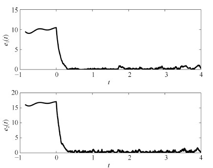
| Fig. 3. The behavior of synchronization error in Example 1. | |
Next,continue to consider Example 1. If the control gains $G_1$,$G_2$ and $G_3$ are not given in advance,the Corollary 2 can be utilized to design the control gains. The detailed procedures will presented below.
First,according to condition (34) and the value of $Q$,we can obtain $G_3$ directly:
$$\begin{align*} G_3 = \left[\begin{array}{cc} -2.4 & 0\\ 0 & -0.75 \end{array}\right]. \end{align*}$$Second,solving LMIs (33) and (35) gives
$$\begin{align*} G_1 = \left[\begin{array}{cc} -14.5930& -2.3084\\ -1.9002& -12.5711 \end{array}\right]& \quad {\rm and} \quad G_2 = \left[\begin{array}{cc} 0 & 0\\ 0 & 0 \end{array}\right]. \end{align*}$$Note that,$G_2 = \bf{0}$,which means the memoryless state feedback controller will also be effective in synchronizing the two MNNs. If we add another condition $G_2<0$ into LMIs \eqref{eq:cor1-condition1} and \eqref{eq:cor1-condition3},we will have:
$$\begin{align*} G_1 = \left[\begin{array}{cc} -9.8929& -2.1042\\ -1.4462& -7.2054 \end{array}\right],\\ G_2 = \left[\begin{array}{cc} -4.4681& -0.4805\\ 0.2420& -3.3275 \end{array}\right]. \end{align*}$$Comparing the two obtained $G_1$,as well as $G_2$,it can be seen that the upper bound of the control gain is reduced,which illustrates Remark 5.
Example 2. Consider the following two-neuron memristive Hopfield neural network model with time delay and additive noise:
| $\begin{align}\label{eq:exm2-model} {\rm d}x = &[-x(t) + A(x)f(x(t)) + B(x)f(x(t-\tau))]{\rm d}t \notag \\ & +\sigma(t,x(t),x(t-\tau)){\rm d}w, \end{align}$ | (59) |
where $x(t)=(x_1(t),x_2(t))^{\rm T}\in {\bf{R}}^2$,$C=I_2$,$\tau=1$,$f(x)=(f_1(x_1),f_2(x_2))^{\rm T}$ with $f_i(x_i)=\tanh(x_i)$ $(i=1,2)$. The weight matrices $A$ and $B$ have the following forms:
$$\begin{align*} A=\left[\begin{array}{cc} 2 & a_{12}(x) \\ a_{21}(x) & 4.5 \end{array} \right]\; {\rm and} \quad B=\left[\begin{array}{cc} -1.5 & -0.1 \\ b_{21}(x) & b_{22}(x) \end{array} \right], \end{align*}$$where
$$\begin{align*} a_{12}(t)&=\left\{\begin{array}{ll} -0.1,& {\rm D}^-f_{11}(t)<0;\\ -0.08,& {\rm D}^-f_{11}(t)>0;\\ a_{12}(t^-),&{\rm D}^-f_{11}(t)=0, \end{array}\right.\\ a_{21}(t)&=\left\{\begin{array}{ll} -5,& {\rm D}^-f_{22}(t)<0;\\ -2.5,& {\rm D}^-f_{22}(t)>0;\\ a_{21}(t^-),& {\rm D}^-f_{22}(t)=0, \end{array}\right.\\ b_{21}(t)&=\left\{\begin{array}{ll} -0.2,& {\rm D}^-f_{11}(t-0.85)<0;\\ 0.1,& {\rm D}^-f_{11}(t-0.85)>0;\\ b_{21}(t^-),& {\rm D}^-f_{11}(t-0.85)=0, \end{array}\right.\\ b_{22}(t)&=\left\{\begin{array}{ll} -4,& {\rm D}^-f_{22}(t-0.85)<0;\\ -3.5,& {\rm D}^-f_{22}(t-0.85)>0;\\ b_{22}(t^-),& {\rm D}^-f_{22}(t-0.85)=0 \end{array}\right. \end{align*}$$and $\sigma(t,x(t),x(t-\tau))$ is given by
$$\begin{align*} \sigma(t,x(t),x(t-\tau)) = \left[\begin{array}{cc} 2x_1(t-1) & 0 \\ 0 & \cos(x_2(t)) \end{array}\right]. \end{align*}$$The controlled response system is described by
| $\begin{align}\label{eq:exm22-model} {\rm d}y = &[-y(t) + A(y)f(y(t)) + B(y)f(y(t-\tau)) \notag \\ &+ u(t)]{\rm d}t +\sigma(t,y(t),y(t-\tau)){\rm d}w, \end{align}$ | (60) |
where $u(t)$ is defined in (43).
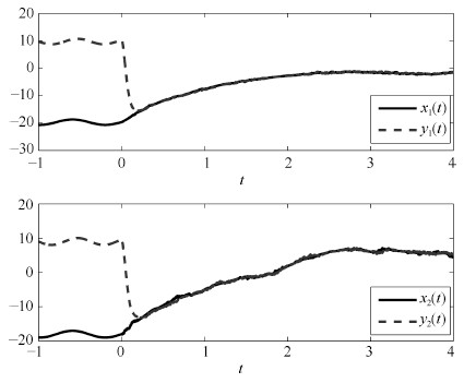
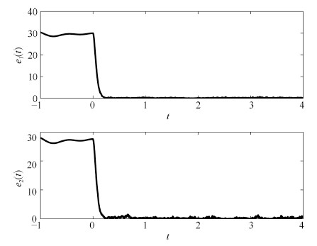
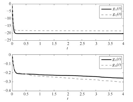
Obviously,the activation functions $f_i(\cdot) (i=1,2)$ satisfy Assumption 1 with $l_1=l_2=1$ and $\gamma_1=\gamma_2=1$. By Theorem (2),RMNN (59) can achieve synchronization in mean square with RMNN (60) under the control law (43). Let $\alpha_1 = \alpha_2 = 0.5$ and $\beta_1=\beta_2=0.1$ in adaptive control law (43). The initial control gains $G_1$ and $G_3$ are both set to be zero. The simulation results are presented in Figs. 4-6.

|
Download:
|
| Fig. 4. Transient behaviors of synchronization via an adaptive control law in Example 2. | |

|
Download:
|
| Fig. 5. The behavior of synchronization error in Example 2. | |

|
Download:
|
| Fig. 6. The behaviors of control gains in Example 2. | |
In this research,the synchronization of two MNNs in the presence of random disturbances is considered. %Two control laws were designed to make the two memristive neural networks with random disturbances achieve global synchronization in mean square. Sufficient conditions were derived based on the stability theory of stochastic differential equations. Finally,two examples were utilized to substantiate the theoretical results. Compared with existing results on synchronization of coupled RMNNs,there are two advantages in this work. First,a state feedback control law utilizing both current and outdated state information is proposed,while only current state information is utilized in the control law in [56]. Such control law can reduce the upper bound of the control gain as illustrated in simulation results. Second,the synchronization criteria depend on two free matrices $\tilde{A}$ and $\tilde{B}$ chosen arbitrarily from an bounded interval,instead of certain fixed matrices (e.g.,the results in [41, 43]. As a result,the synchronization criteria here are less conservative. In addition,the approach for computing the control gains is given.
Many avenues are open for future research on the synchronization problems of MNNs with random disturbances. Further investigations may aim at analyzing impulsive synchronization,sample-date synchronization,intermittence synchronization,quantization synchronization and lag synchronization of driving-response MNNs and multi-coupled MNNs in the presence of random disturbances.
| [1] | Chua L O. Memristor-the missing circuit element. IEEE Transactions on Circuit Theory, 1971, 18(5): 507-519 |
| [2] | Mathur N D. The fourth circuit element. Nature, 2008, 455(7217): E13 |
| [3] | Strukov D B, Snider G S, Stewart D R, Williams R S. The missing memristor found. Nature, 2008, 453(7191): 80-83 |
| [4] | Itoh M, Chua L O. Memristor cellular automata and memristor discretetime cellular neural networks. International Journal of Bifurcation and Chaos, 2009, 19(11): 3605-3656 |
| [5] | Pershin Y V, Di Ventra M. Experimental demonstration of associative memory with memristive neural networks. Neural Networks, 2010, 23(7): 881-886 |
| [6] | Cao J D, Wang J. Global asymptotic stability of a general class of recurrent neural networks with time-varying delays. IEEE Transactions on Circuits and Systems I: Fundamental Theory and Applications, 2003, 50(1): 34-44 |
| [7] | Cao J D, Wang J. Global asymptotic and robust stability of recurrent neural networks with time delays. IEEE Transactions on Circuits and Systems I: Regular Papers, 2005, 52(2): 417-426 |
| [8] | Wang Z S, Zhang H G, Jiang B. LMI-based approach for global asymptotic stability analysis of recurrent neural networks with various delays and structures. IEEE Transactions on Neural Networks, 2011, 22(7): 1032-1045 |
| [9] | Zhang H G, Wang Z S, Liu D R. A comprehensive review of stability analysis of continuous-time recurrent neural networks. IEEE Transactions on Neural Networks and Learning Systems, 2014, 25(7): 1229-1262 |
| [10] | Wang Z S, Liu L, Shan Q H, Zhang H G. Stability criteria for recurrent neural networks with time-varying delay based on secondary delay partitioning method. IEEE Transactions on Neural Networks and Learning Systems, 2015, 26(10): 2589-2595 130 IEEE/CAA JOURNAL OF AUTOMATICA SINICA, VOL. 3, NO. 2, APRIL 2016 |
| [11] | Wang Z, Ding S, Huang Z, Zhang H. Exponential stability and stabilization of delayed memristive neural networks based on quadratic convex combination method. IEEE Transactions on Neural Networks and Learning Systems, 2015, 1-14 |
| [12] | Hu J, Wang J. Global uniform asymptotic stability of memristor-based recurrent neural networks with time delays. In: Proceedings of the 2010 International Joint Conference on Neural Networks (IJCNN). Barcelona: IEEE, 2010. 1-8 |
| [13] | Wu A L, Zeng Z G. Dynamic behaviors of memristor-based recurrent neural networks with time-varying delays. Neural Networks, 2012, 36: 1-10 |
| [14] | Wen S P, Zeng Z G, Huang T W. Exponential stability analysis of memristor-based recurrent neural networks with time-varying delays. Neurocomputing, 2012, 97: 233-240 |
| [15] | Guo Z Y, Wang J, Yan Z. Global exponential dissipativity and stabilization of memristor-based recurrent neural networks with time-varying delays. Neural Networks, 2013, 48: 158-172 |
| [16] | Guo Z Y, Wang J, Yan Z. Attractivity analysis of memristor-based cellular neural networks with time-varying delays. IEEE Transactions on Neural Networks and Learning Systems, 2014, 25(4): 704-717 |
| [17] | Guo Z Y, Wang J, Yan Z. Passivity and passification of memristor-based recurrent neural networks with time-varying delays. IEEE Transactions on Neural Networks and Learning Systems, 2014, 25(11): 2099-2109 |
| [18] | Pecora L M, Carroll T L. Synchronization in chaotic systems. Physical Review Letters, 1990, 64(8): 821-824 |
| [19] | Hansel D, Sompolinsky H. Synchronization and computation in a chaotic neural network. Physical Review Letters, 1992, 68(5): 718-721 |
| [20] | Hoppensteadt F C, Izhikevich E M. Pattern recognition via synchronization in phase-locked loop neural networks. IEEE Transactions on Neural Networks, 2000, 11(3): 734-738 |
| [21] | Chen G R, Zhou J, Liu Z R. Global synchronization of coupled delayed neural networks and applications to chaotic CNN models. International Journal of Bifurcation and Chaos, 2004, 14(7): 2229-2240 |
| [22] | Lu W, Chen T. Synchronization of coupled connected neural networks with delays. IEEE Transactions on Circuits and Systems I: Regular Papers, 2004, 51(12): 2491-2503 |
| [23] | Wu W, Chen T P. Global synchronization criteria of linearly coupled neural network systems with time-varying coupling. IEEE Transactions on Neural Networks, 2008, 19(2): 319-332 |
| [24] | Liang J L, Wang Z D, Liu Y R, Liu X H. Global synchronization control of general delayed discrete-time networks with stochastic coupling and disturbances. IEEE Transactions on Systems, Man, and Cybernetics, Part B: Cybernetics, 2008, 38(4): 1073-1083 |
| [25] | Yu W W, Chen G R, Lu J H. On pinning synchronization of complex dynamical networks. Automatica, 2009, 45(2): 429-435 |
| [26] | Lu J Q, Ho D W C, Cao J D. A unified synchronization criterion for impulsive dynamical networks. Automatica, 2010, 46(7): 1215-1221 |
| [27] | Liu T, Zhao J, Hill D J. Exponential synchronization of complex delayed dynamical networks with switching topology. IEEE Transactions on Circuits and Systems I: Regular Papers, 2010, 57(11): 2967-2980 |
| [28] | Zhang W B, Tang Y, Miao Q Y, Du W. Exponential synchronization of coupled switched neural networks with mode-dependent impulsive effects. IEEE Transactions on Neural Networks and Learning Systems, 2013, 24(8): 1316-1326 |
| [29] | Wu L G, Feng Z G, Lam J. Stability and synchronization of discrete-time neural networks with switching parameters and time-varying delays. IEEE Transactions on Neural Networks and Learning Systems, 2013, 24(12): 1957-1972 |
| [30] | Tang Y, Wai K W. Distributed synchronization of coupled neural networks via randomly occurring control. IEEE Transactions on Neural Networks and Learning Systems, 2013, 24(3): 435-447 |
| [31] | Liu Y R, Wang Z D, Liang J L, Liu X H. Synchronization of coupled neutral-type neural networks with jumping-mode-dependent discrete and unbounded distributed delays. IEEE Transactions on Cybernetics, 2013, 43(1): 102-114 |
| [32] | Cao J D, Chen G R, Li P. Global synchronization in an array of delayed neural networks with hybrid coupling. IEEE Transactions on Systems, Man, and Cybernetics, Part B: Cybernetics, 2008, 38(2): 488-498 |
| [33] | Lu H T, van Leeuwen C. Synchronization of chaotic neural networks via output or state coupling. Chaos, Solitons & Fractals, 2006, 30(1): 166-176 |
| [34] | Cao J D, Lu J Q. Adaptive synchronization of neural networks with or without time-varying delay. Chaos, 2006, 16(1): 013133 |
| [35] | Wu Z G, Shi P, Su H Y, Chu J. Sampled-data synchronization of chaotic Lur'e systems with time delays. IEEE Transactions on Neural Networks and Learning Systems, 2013, 24(3): 410-421 |
| [36] | Zhang H G, Ma T D, Huang G B, Wang Z X. Robust global exponential synchronization of uncertain chaotic delayed neural networks via dual-stage impulsive control. IEEE Transactions on Systems, Man, and Cybernetics, Part B: Cybernetics, 2010, 40(3): 831-844 |
| [37] | Wu A L, Wen S P, Zeng Z G. Synchronization control of a class of memristor-based recurrent neural networks. Information Sciences, 2012, 183(1): 106-116 |
| [38] | Zhang G D, Shen Y. New algebraic criteria for synchronization stability of chaotic memristive neural networks with time-varying delays. IEEE Transactions on Neural Networks and Learning Systems, 2013, 24(10): 1701-1707 |
| [39] | Wen S P, Bao G, Zeng Z G, Chen Y R, Huang T W. Global exponential synchronization of memristor-based recurrent neural networks with timevarying delays. Neural Networks, 2013, 48: 195-203 |
| [40] | Zhang G D, Shen Y. Exponential synchronization of delayed memristorbased chaotic neural networks via periodically intermittent control. Neural Networks, 2014, 55: 1-10 |
| [41] | Yang X S, Cao J D, Yu W W. Exponential synchronization of memristive Cohen-Grossberg neural networks with mixed delays. Cognitive Neurodynamics, 2014, 8(3): 239-249 |
| [42] | Chen J J, Zeng Z G, Jiang P. Global Mittag-Leffler stability and synchronization of memristor-based fractional-order neural networks. Neural Networks, 2014, 51: 1-8 |
| [43] | Guo Z Y, Wang J, Yan Z. Global exponential synchronization of two memristor-based recurrent neural networks with time delays via static or dynamic coupling. IEEE Transactions on Systems, Man, and Cybernetics: Systems, 2015, 45(2): 235-249 |
| [44] | Guo Z Y, Yang S F, Wang J. Global exponential synchronization of multiple memristive neural networks with time delay via nonlinear coupling. IEEE Transactions on Neural Networks and Learning Systems, 2015, 26(6): 1300-131132 |
| [45] | Yang S F, Guo Z Y, Wang J. Robust synchronization of multiple memristive neural networks with uncertain parameters via nonlinear coupling. IEEE Transactions on Systems, Man, and Cybernetics: Systems, 2015, 45(7): 1077-1086 |
| [46] | Tuckwell H C. Stochastic Processes in the Neurosciences. Philadelphia, PA: SIAM, 1989. |
| [47] | Haykin S. Kalman Filtering and Neural Networks. New York: Wiley, 2001. |
| [48] | Huang H, Ho D W C, Lam J. Stochastic stability analysis of fuzzy Hopfield neural networks with time-varying delays. IEEE Transactions on Circuits and Systems II: Express Briefs, 2005, 52(5): 251-255 |
| [49] | Wang Z D, Liu Y R, Li M Z, Liu X H. Stability analysis for stochastic Cohen-Grossberg neural networks with mixed time delays. IEEE Transactions on Neural Networks, 2006, 17(3): 814-820 |
| [50] | Liang J L, Wang Z D, Liu Y R, Liu X H. Robust synchronization of an array of coupled stochastic discrete-time delayed neural networks. IEEE Transactions on Neural Networks, 2008, 19(11): 1910-1921 |
| [51] | Wang Z D, Wang Y, Liu Y R. Global synchronization for discrete-time stochastic complex networks with randomly occurred nonlinearities and mixed time delays. IEEE Transactions on Neural Networks, 2010, 21(1): 11-25 |
| [52] | Huang C X, Cao J D. Convergence dynamics of stochastic Cohen- Grossberg neural networks with unbounded distributed delays. IEEE Transactions on Neural Networks, 2011, 22(4): 561-572 |
| [53] | Lu J Q, Kurths J, Cao J D, Mahdavi N, Huang C. Synchronization control for nonlinear stochastic dynamical networks: pinning impulsive strategy. IEEE Transactions on Neural Networks and Learning Systems, 2012, 23(2): 285-292 |
| [54] | Zhang W B, Tang Y, Miao Q Y, Fang J A. Synchronization of stochastic dynamical networks under impulsive control with time delays. IEEE Transactions on Neural Networks and Learning Systems, 2014, 25(10): 1758-1768 |
| [55] | Yang X S, Cao J D, Qiu J L. pth moment exponential stochastic synchronization of coupled memristor-based neural networks with mixed delays via delayed impulsive control. Neural Networks, 2015, 65: 80-91 |
| [56] | Ding S B, Wang Z S. Stochastic exponential synchronization control of memristive neural networks with multiple time-varying delays. Neurocomputing, 2015, 162: 16-25 |
| [57] | Øksendal B. Stochastic Differential Equations. Berlin Heidelberg: Springer, 2003. |
| [58] | Chua L. Resistance switching memories are memristors. Applied Physics A, 2011, 102(4): 765-783 |
| [59] | Jo S H, Chang T, Ebong I, Bhadviya B B, Mazumder P, Lu W. Nanoscale memristor device as synapse in neuromorphic systems. Nano Letters, 2010, 10(4): 1297-1301 |
| [60] | Sah M P, Yang C J, Kim H, Chua L. A voltage mode memristor bridge synaptic circuit with memristor emulators. Sensors, 2012, 12(3): 3587-3604 |
| [61] | Kim H, Sah M P, Yang C J, Roska T, Chua L O. Neural synaptic weighting with a pulse-based memristor circuit. IEEE Transactions on Circuits and Systems I: Regular Papers, 2012, 59(1): 148-158 |
| [62] | Adhikari S P, Yang C J, Kim H, Chua L O. Memristor bridge synapsebased neural network and its learning. IEEE Transactions on Neural Networks and Learning Systems, 2012, 23(9): 1426-1435 |
| [63] | Boyd S, El Ghaoui L, Feron E, Balakrishnan B. Linear Matrix Inequalities in System and Control Theory. Philadelphia: SIAM, 1994. |
| [64] | Edwards C, Spurgeon S K, Patton R J. Sliding mode observers for fault detection and isolation. Automatica, 2000, 36(4): 541-553 |