 2016, Vol.3


IN the past several decades,the control methods for uncertain nonlinear system have received much attention and a lot of results have been achieved,such as adaptive feedback linearization technique,adaptive backstepping technique,fuzzy control and neural network control etc.[1, 2, 3, 4, 5, 6, 7, 8, 9],but most of the studies are based on affine systems in which the control inputs appear in a linear fashion. In practice,there are many nonlinear systems with non-affine structure in which the control inputs are embedded nonlinearly into the system through various possible ways[10, 11, 12],such as chemical reactors,biochemical process,aircraft dynamics,dynamic model in pendulum control etc. Control design for non-affine systems has become an innovative and challenging topic,and some remarkable results have been obtained. Generally,the studies for the control problem of non-affine system can be broadly classified in three categories.
In the first category,the control methods are focused on transforming the original system non-affine into a new system in which the new control input variable appears in an affine form. There are three ways of transforming the non-affine into affine-like form,such as: 1) using Taylor series expansion to transform the original non-affine system into the affine-like one in the neighborhood of the operating trajectory[13, 14, 15]; 2) by employing the mean value theorem to transform the non-affine into affine-like form[16, 17]; 3) by differentiating the original nonlinear state equation once such that the resulting augmented state equation is linear in the new control variable,i.e. the derivative of the control input[11, 18]. Note that most of these schemes are based on some idealized assumptions,namely the sign of the control gain which represents motion direction of the system under any control is known,the non-affine function is known a priori,the partial derivatives of nonlinear functions are known and the partial derivatives of nonlinear functions are bounded,etc.. In the second category,the implicit function theorem is used to demonstrate the existence of an ideal control input for the non-affine system[19, 20, 21, 22, 23, 24]. Since it is difficult to invert the non-affine nonlinearities to get an explicit inverting control input,the implicit function theorem does not provide a way for determining such inverting control input. In this situation,some works combine implicit function theorem with neural networks (NN)[20, 21, 22, 23] and fuzzy logic system (FLS)[24, 25] which are used to approximate the ideal control input. Similar to the first category,these schemes are also based on some idealized assumptions,for example,the sign of the control gain is also known. In the third category,the Lyapunov direct method is proposed[26, 27]. This method does not need to transform the non-affine into affine or use the implicit function theorem,but must seek out an adaptive Lyapunov function. Unfortunately,it is very difficult to seek out a proper Lyapunov function and this method can not usually process the uncertain system.
Nowadays,backstepping technique has become a powerful control method for uncertain nonlinear systems [6, 7, 8]. The design procedure treats the state variables as virtual control inputs,step by step to design the virtual controllers and illustrates the stability by Lyapunov stability theorem,then the actual control input can be obtained. However,a drawback with the backstepping technique is the problem of “explosion of complexity” [23, 28, 29, 30, 31, 32]. Inspired by the above researches,in this paper,an adaptive robust control scheme will be proposed for a class of uncertain MIMO non-affine nonlinear system. Compared with the existing literature,the following contributions are worth to be emphasized.
1) To overcome the non-affine difficulty,mean value theorem is employed to transform the systems into the affine-like form. In contrast with the existing results such as [16, 17, 18],the proposed control scheme not only transforms the systems into the affine-like form,but also simplifies the assumptions,such as it only needs partial derivatives $\frac{\partial f( \cdot )}{\partial x}$ are bounded on known constant closed intervals,and the control scheme is independent of function $f( \cdot )$ and the partial derivatives functions $\frac{\partial f( \cdot )}{\partial x}$ and $\frac{\partial f( \cdot )}{\partial u}$.
2) The bounded time-varying parameters are estimated by adaptive algorithms with projection,the estimation error and external disturbance are compensated by employing nonlinear damping technique,Compared with the existing literatures such as [16, 17, 18, 19, 20, 21, 22, 23, 24],the proposed control scheme does not need any NN or FLS approximation,which reduces dramatically the number of online learning parameters.
3) By combining dynamic surface control (DSC) with Nussbaum function,the control scheme can not only overcome the ``explosion of complexity'' problem but also deal with the possible ``controller singularity'' problem [16, 33, 34, 35]. Thus,the proposed control scheme reduces the computation load of the algorithm correspondingly and makes it easy in actual implementation.
The organization of the paper is as follows: The problem formulation is presented in Section II. A design procedure for adaptive robust control is established in Section III. An analysis procedure for stability and tracking performance of the closed-loop system is developed in Section IV. The promising results of the proposed method are demonstrated through simulation in Section V. Finally,the paper is concluded in Section VI.
II. PROBLEM FORMULATION AND PRELIMINARY A.Problem FormulationConsider a class of uncertain MIMO non-affine nonlinear systems with uncertain structure and parameters,unknown control direction and unknown external disturbance which is described by
| $\left\{ \begin{array}{*{35}{l}} {{{\dot{x}}}_{i}}={{f}_{i}}({{{\bar{x}}}_{i}},{{x}_{i+1}})+{{\Delta }_{i}}({{{\bar{x}}}_{i}},t),\\ {{{\dot{x}}}_{n}}={{f}_{n}}({{{\bar{x}}}_{n}},u)+{{\Delta }_{n}}({{{\bar{x}}}_{n}},t),\\ y={{x}_{1}},\\ \end{array} \right.$ | (1) |
where $x_i = [x_{i1} ,\ldots ,x_{im}]^{\rm T} \in {\bf R}^m$,$\bar x_i =[x_1^{\rm T} ,\ldots ,x_i^{\rm T}]^{\rm T} $,$i = 1,2,\ldots n$,$u \in {\bf R}^m$ and $y \in {\bf R}^m$ are the system states,input and output respectively. $f_i ( \cdot ) =$ $[f_{i1} ( \cdot ),f_{i2} ( \cdot ),\ldots ,f_{im} ( \cdot )]^{\rm T}$ is a smooth nonlinear function with uncertain structure and parameters. $\Delta _i (\bar x_i ,t) =$ $[\Delta _{i1} (\bar x_i ,t),\Delta _{i2} (\bar x_i ,t),\ldots ,\Delta _{im} (\bar x_i ,t)]^{\rm T}$ denotes the external disturbance. To facilitate the control system design,let $x_{n + 1} = u$ and define
$\begin{align} & {{G}_{ij}}=\frac{\partial {{f}_{i}}({{{\bar{x}}}_{i}},{{x}_{i+1}})}{\partial {{x}_{j}}}=\left[\begin{matrix} \frac{\partial {{f}_{i1}}(\cdot )}{\partial {{x}_{j1}}} & \ldots & \frac{\partial {{f}_{i1}}(\cdot )}{\partial {{x}_{jm}}} \\ \vdots & \ddots & \vdots \\ \frac{\partial {{f}_{im}}(\cdot )}{\partial {{x}_{j1}}} & \ldots & \frac{\partial {{f}_{im}}(\cdot )}{\partial {{x}_{jm}}} \\ \end{matrix} \right],\\ & \qquad \qquad \qquad \qquad \ i=1,2,\ldots ,n,\ j=1,2,\ldots ,i,\\ & {{G}_{xi}}=\frac{\partial {{f}_{i}}({{{\bar{x}}}_{i}},{{x}_{i+1}})}{\partial {{{\bar{x}}}_{i}}}=\left[\frac{\partial {{f}_{i}}(\cdot )}{\partial {{x}_{1}}},\ldots ,\frac{\partial {{f}_{i}}(\cdot )}{\partial {{x}_{i}}} \right] \\ & \quad \ =[{{G}_{i1}},{{G}_{i2}},\ldots ,{{G}_{ii}}],\quad i=1,2,\ldots ,n,\\ & {{G}_{ui}}=\frac{\partial {{f}_{i}}({{{\bar{x}}}_{i}},{{x}_{i+1}})}{\partial {{x}_{i+1}}}=\left[\begin{matrix} \frac{\partial {{f}_{i1}}(\cdot )}{\partial {{x}_{(i+1)1}}} & \ldots & \frac{\partial {{f}_{i1}}(\cdot )}{\partial {{x}_{(i+1)m}}} \\ \vdots & \ddots & \vdots \\ \frac{\partial {{f}_{im}}(\cdot )}{\partial {{x}_{(i+1)1}}} & \ldots & \frac{\partial {{f}_{im}}(\cdot )}{\partial {{x}_{(i+1)m}}} \\ \end{matrix} \right],\\ & \qquad \qquad \qquad \qquad \qquad \qquad \qquad \qquad \ i=1,2,\ldots ,n,\\ & {{g}_{ijlk}}=\frac{\partial {{f}_{il}}({{{\bar{x}}}_{i}},{{x}_{i+1}})}{\partial {{x}_{jk}}},\qquad \ \\ & i=1,2,\ldots ,n,\ j=1,2,\ldots ,i+1,\ l,k=1,2,\ldots ,m. \\ \end{align}$
In this paper,the control objective is that the adaptive robust control scheme is developed for the system (1),such that the system output $y$ converges to a small neighborhood of the reference signal $y_r$ in the presence of uncertain structure and parameters,unknown control direction and unknown external disturbance. To design appropriate controller for the system (1),the following assumptions are imposed.
Assumption 1. For the uncertain MIMO nonlinear system(1),nonlinear function $f_i( \cdot )$ is continuously differentiable and the partial derivatives $\frac{\partial f_i( \cdot )}{\partial x_j}$,$i = 1,\ldots ,n$,$j = 1,\ldots ,i + 1$ are bounded on known constant closed intervals. Namely each element of $G_{ij}$ is confined to a certain range ${{g}_{ijlk}}\in [{{\underset{\raise0.3em\hbox{$\smash{\scriptscriptstyle-}$}}{g}}_{ijlk}},{{\bar{g}}_{ijlk}}]$,where $\underline g_{ijlk}$ and $\bar g_{ijlk}$ are known constants,that is,there exist known constant matrices $\underline G_{xi}$,$\underline G_{ui}$,$\bar G_{xi} $, $\bar G_{ui} $,such that $\underline G_{xi} \le G_{xi}\le \bar G_{xi}$ and $\underline G_{ui} \le G_{ui} \le \bar G_{ui}$.
Assumption 2.For the uncertain MIMO nonlinear system (1),the initial value of $f_i(\cdot)$ is bounded by a positive constant $d_0$,i.e., $\left| {f_{il} (0,\ldots ,0)} \right| \le d_0 $, $l = 1,2,\ldots,m$.
Assumption 3.For the uncertain MIMO nonlinear system(1),the external disturbance $\Delta _i (\bar x_i ,t) = [\Delta _{i1} (\bar x_i ,t),\Delta _{i2}$ $(\bar x_i ,t),$ $\ldots ,\Delta _{im} (\bar x_i ,t)]^{\rm T}$ satisfies $\left\| {\Delta _i (\bar x_i ,t)} \right\| \le \rho _i (\bar x_i )f_{di} (t)$ and $\left| {f_{di} (t)} \right| \le d_i$,where $\rho _i (\bar x_i )$ is a known smooth function and $d_i$ is a positive constant.
Assumption 4. For the uncertain MIMO nonlinear system(1),the desired trajectory $y_r(t)$,$\dot y_r (t)$ and $\ddot y_r (t)$ are continuous and bounded,that is,there exists a constant $C_0 > 0$,such that $\Pi _0 = \{ (y_r ,\dot y_r ,\ddot y_r ):\left\| {y_r } \right\|^2 + \left\| {\dot y_r } \right\|^2 + \left\| {\ddot y_r } \right\|^2 \le C_0 \}$.
By adding and subtracting term $ f_i ({\bf{0}},{\bf{0}},\ldots,{\bf{0}})$,$f_i$ can be written as
| $\begin{align} & {{f}_{i}}({{{\bar{x}}}_{i}},{{x}_{i+1}}) \\ & \qquad ={{f}_{i}}({{{\bar{x}}}_{i}},{{x}_{i+1}})-{{f}_{i}}(\mathbf{0},{{x}_{2}},\ldots ,{{x}_{i}},{{x}_{i+1}})\text{ } \\ & \qquad \quad +{{f}_{i}}(\mathbf{0},{{x}_{2}},\ldots ,{{x}_{i}},{{x}_{i+1}})-{{f}_{i}}(\mathbf{0},\mathbf{0},{{x}_{3}},\ldots ,{{x}_{i}},{{x}_{i+1}}) \\ & \qquad \quad +\cdots \text{ } \\ & \qquad \quad +{{f}_{i}}(\mathbf{0},\ldots ,\mathbf{0},{{x}_{i+1}})-{{f}_{i}}(\mathbf{0},\ldots ,\mathbf{0},\mathbf{0}) \\ & \qquad \quad +{{f}_{i}}(\mathbf{0},\mathbf{0},\ldots ,\mathbf{0}).\text{ } \\ \end{align}$ | (2) |
Since $f_i$ is continuously differentiable,$f_i$ can be written further as following form by using the mean value theorem.
| $ \begin{align} & {{f}_{i}}({{{\bar{x}}}_{i}},{{x}_{i+1}})=\left( {{\left. \frac{\partial {{f}_{i}}({{{\bar{x}}}_{i}},{{x}_{i+1}})}{\partial {{x}_{1}}} \right|}_{({{\gamma }_{1}},{{x}_{2}},\ldots ,{{x}_{i+1}})}} \right){{x}_{1}} \\ & \qquad +\left( {{\left. \frac{\partial {{f}_{i}}({{{\bar{x}}}_{i}},{{x}_{i+1}})}{\partial {{x}_{2}}} \right|}_{(0,{{\gamma }_{2}},{{x}_{3}},\ldots ,{{x}_{i+1}})}} \right){{x}_{2}}+\cdots \\ & \ +\left( {{\left. \frac{\partial {{f}_{i}}({{{\bar{x}}}_{i}},{{x}_{i+1}})}{\partial {{x}_{i}}} \right|}_{(0,\ldots ,0,{{\gamma }_{j}},{{x}_{i+1}})}} \right){{x}_{i}} \\ & \ +\left( {{\left. \frac{\partial {{f}_{i}}({{{\bar{x}}}_{i}},{{x}_{i+1}})}{\partial {{x}_{i+1}}} \right|}_{(0,\ldots ,0,{{\gamma }_{j+1}})}} \right){{x}_{i+1}}+{{f}_{i}}(\mathbf{0})\text{ } \\ & =\ \sum\limits_{j=1}^{i}{\left( {{\left. \frac{\partial {{f}_{i}}({{{\bar{x}}}_{i}},{{x}_{i+1}})}{\partial {{x}_{j}}} \right|}_{(\mathbf{0},{{\gamma }_{j}},{{x}_{i+1}})}} \right)}{{x}_{j}}\text{ } \\ & \ +{{\left. \frac{\partial {{f}_{i}}({{{\bar{x}}}_{i}},{{x}_{i+1}})}{\partial {{x}_{i+1}}} \right|}_{(\mathbf{0},{{\gamma }_{j+1}})}}{{x}_{i+1}}+{{f}_{i}}(\mathbf{0})\text{ } \\ & =\ {{G}_{xi}}{{{\bar{x}}}_{i}}+{{G}_{ui}}{{x}_{i+1}}+{{f}_{i}}(\mathbf{0}),\\ \end{align} $ | (3) |
where $f_i(0)$ is the abbreviation for $f_i ({\bf{0}},{\bf{0}}, \ldots,{\bf{0}})$. and
${{g}_{ijlk}}=\frac{\partial {{f}_{il}}({{{\bar{x}}}_{i}},{{x}_{i+1}})}{\partial {{x}_{jk}}}\left| \begin{matrix} (\{0,\ldots ,0\},\ldots ,\\ \begin{matrix} \{{{\gamma }_{j1}},\ldots ,{{\gamma }_{jk}}\},\ldots ,\\ \{{{x}_{(i+1)1}},\ldots ,{{x}_{(i+1)k}}\}) \\ \end{matrix} \\ \end{matrix} \right.,$
where $\gamma _{jk} \in [0,x_{(j - 1)k}]$,$j = 1,2,\ldots ,i + 1$ and $k=1,2,\ldots ,m$. the time-varying matrices $g_{xi}$ and $g_{ui}$ are bounded and satisfy assumption 1. so system (1) can be transformed into a time-varying system with strict feedback structure,and it follows that
| $ \begin{align} \begin{cases} \dot x_i = G_{xi} \bar x_i + G_{ui} x_{i + 1} + f_i ({\bf{0}}) + \Delta _i (\bar x_i ,t),\\ \qquad\qquad\qquad\qquad\qquad i = 1,2,\ldots ,n - 1 ,\\ \dot x_n = G_{xn} \bar x_n + G_{un} u + f_n ({\bf{0}})+ \Delta _n (\bar x_n ,t),\\ y = x_1. \end{cases} \end{align} $ | (4) |
In order to deal with the unknown sign of control gain matrix $G_{ui}$,the Nussbaum gain technique is employed in this paper. A function $N(\tau)$ is called Nussbaum-type function if it has the following properties
| $$\left\{ \begin{array}{*{35}{l}} \underset{s\to +\infty }{\mathop{\lim }}\,\sup \frac{1}{s}\int\limits_{0}^{s}{N(\tau )\text{d}\tau =+\infty },\\ \underset{s\to +\infty }{\mathop{\lim }}\,\inf \frac{1}{s}\int\limits_{0}^{s}{N(\tau )\text{d}\tau =+\infty }. \\ \end{array} \right. $$ | (5) |
In this paper,$N(\tau ) = \tau ^2 \cos (\tau )$ will be exploited. In the stability analysis,we need the following lemmas.
Lemma 1 [16, 33, 34]. Let $V(\cdot)$ and $\tau (\cdot)$ be smooth functions defined on $[0,t_f )$ with $V(t) \ge 0$,$\forall t \in [0,t_f )$ and $N(\cdot)$ is an even smooth Nussbaum-type function. If the following inequality holds,the $V(t)$,$\tau (t)$ and $\int_0^t {(a(x(\kappa ))N(\tau )} + 1)\dot \tau {\rm d}\tau$ must be bounded on $[0,t_f )$.
| $\begin{array}{*{35}{l}} 0 & \le V(t)\text{ } \\ {} & \le {{b}_{0}}+{{\text{e}}^{-{{b}_{1}}t}}\int_{0}^{t}{(a(x(\kappa ))N(\tau )+1)\dot{\tau }{{\text{e}}^{{{b}_{1}}t}}\text{d}\kappa },\ \forall t\in [0,{{t}_{f}}),\\ \end{array} $ | (6) |
where $b_0$ represents some suitable constant,$b_1$ is a positive constant,and $a(x(\kappa )$ is a time-varying parameter which takes values in the unknown closed intervals $\Re =[I^ - ,I^ +]$,with $0\notin \Re $.
Lemma 2
Let $\hat \theta$ be an estimate of $\theta$,$\tilde \theta = \theta - \hat \theta$ denotes the parameters projection errors. In this paper,the following adaptive algorithm with projection will be exploited[11, 36].
| $\begin{align} & \dot{\hat{\theta }}=\Pr \text{o}{{\text{j}}_{{\hat{\theta }}}}(\Gamma \varsigma ),\ \ \hat{\theta }(0)\in {{\Omega }_{\theta }},\\ & \Pr \text{o}{{\text{j}}_{{\hat{\theta }}}}(\cdot i)=\left\{ \begin{array}{*{35}{l}} 0,& \hat{\theta }={{\theta }_{\max }},\ \cdot i>0,\\ 0,& \hat{\theta }={{\theta }_{\min }},\ \cdot i<0,\\ \cdot i,& \text{other},\\ \end{array} \right. \\ \end{align} $ | (7) |
where $\Omega _\theta$ is the closed interval $[\theta _{\min } ,\theta _{\max }]$,$\Gamma $ is a diagonal matrix,and $\varsigma$ is an adaptive function. It follows that the adaptive algorithm with projection assures that $\forall t:\hat \theta (t) \in \Omega _\theta$ is satisfied for all values of arguments.
III. DESIGN OF ADAPTIVE ROBUST CONTROLLERIn this section,we will establish an adaptive DSC design scheme for the uncertain MIMO non-affine nonlinear system (1). Similar to the traditional backstepping adaptive control design methods,the recursive design procedure contains $n$ steps.
Step 1. For the first subsystem of system (1),defining ${{S}_{1}}={{x}_{1}}-{{y}_{r}},{{S}_{1}}={{[{{S}_{11}},{{S}_{12}},\ldots ,{{S}_{1m}}]}^{\text{T}}}$ and differentiating $S_1$ with respect to time yields
| $\begin{array}{*{35}{l}} {{{\dot{S}}}_{1}} & ={{{\dot{x}}}_{1}}-{{{\dot{y}}}_{r}}\text{ } \\ {} & ={{G}_{x1}}{{{\bar{x}}}_{1}}+{{G}_{u1}}{{x}_{2}}+{{\Delta }_{1}}+{{f}_{1}}(\mathbf{0})-{{{\dot{y}}}_{r}},\\ \end{array} $ | (8) |
where $\Delta _1$ is the abbreviation for $\Delta _1 (x_1 ,t) $. Defining ${{\Psi }_{1}}={{[{{G}_{x1}},{{f}_{1}}(\mathbf{0}),{{I}_{m\times m}}]}^{\text{T}}}$,$\Upsilon _1 = [\bar x_1^{\rm T} ,1,- \dot y_r^{\rm T}]^{\rm T}$,$\dot S_1$ can be rewritten as
| $\begin{align} \dot S_1 = G_{u1} x_2 + \Psi _1^{\rm T} \Upsilon _1 + \Delta _1, \end{align} $ | (9) |
where $x_2$ is viewed as the virtual control variable. For the first subsystem of system (1),we consider the following virtual control law $x_{2r}$ which incorporates the Nussbaum function.
| $\begin{align} \begin{cases} x_{2r} = N(\tau _1 )(K_1 S_1 + \hat \Psi _1^{\rm T} \Upsilon _1 + \vartheta _1 ),\\ N(\tau _1 ) = \tau _1^2 \cos (\tau _1 ),\\ \vartheta _1 = \left(\frac {\zeta _1^2}{4\gamma _1} + \rho _1^2 \frac{\bar x_1 }{4\chi _1}\right) \cdot S_1,\\ \end{cases} \end{align} $ | (10) |
where
$\begin{align} & {{\zeta }_{1}}\ge \left\| {{{\tilde{\Psi }}}_{1\max }} \right\|\left\| {{\Upsilon }_{1}} \right\|,\ \ {{{\tilde{\Psi }}}_{1\max }}={{\Psi }_{1\max }}-{{\Psi }_{1\min }},\\ & {{\Psi }_{1\max }}={{[{{{\bar{G}}}_{x1}},{{D}_{1}},{{I}_{m\times m}}]}^{\text{T}}},\\ & {{\Psi }_{1\min }}={{[{{{\underset{\raise0.3em\hbox{$\smash{\scriptscriptstyle-}$}}{G}}}_{x1}},-{{D}_{1}},-{{I}_{m\times m}}]}^{\text{T}}},\\ & {{D}_{1}}={{[\underbrace{{{d}_{0}},{{d}_{0}},\ldots ,{{d}_{0}}}_{m}]}^{\text{T}}},\\ \end{align}$
the adaptation law for $\tau_1$ and $\hat \Psi _1$ are chosen as
| $\begin{align} \begin{cases} \dot \tau _1 = S_1^{\rm T} (K_1 S_1 + \hat \Psi _1^{\rm T} \Upsilon _1 + \vartheta _1 ),\\ \dot {\hat{ \Psi}} _{1}= \Pr {\rm{oj}}_{\hat \Psi 1} (\Gamma _{\Psi 1} \Upsilon _1 S_1^{\rm T} ),\ \ \hat \Psi _{10} \in \Omega _{\Psi 1} , \end{cases} \end{align} $ | (11) |
where $\Omega _{\Psi 1}$ is the closed interval $[\Psi _{1\min},\Psi _{1\max }]$,the item $\vartheta _1$ is used to compensate projection error $\tilde \Psi _1 = \Psi _1 - \hat \Psi _1$ and external disturbance $\Delta _1$. Design parameters $K_1$,$\gamma _1$ and $\chi _1$ are chosen as positive constants,and design parameter $\Gamma _{\Psi 1}$ is a positive constant diagonal matrix. To avoid repeatedly differentiating the virtual control law,the DSC method is applied. Namely,make the virtual control law $x_{2r}$ pass through a first-order filter
| $\begin{align} &\mu _2 \dot z_2 + z_2 = x_{2r} ,\ \ z_2 (0) = x_{2r} (0), \end{align} $ | (12) |
where $\mu _2 > 0$ is the time constant of the first-order filter.
Step i(i=2,...,n-1). Defining $S_i = x_i - z_i$,${{S}_{i}}={{[{{S}_{i1}},{{S}_{i2}},\ldots ,{{S}_{im}}]}^{\text{T}}}$ and differentiating $S_i$ with respect to time yields
| $\begin{align} \dot S_i = G_{xi} \bar x_i + G_{ui} x_{i + 1} + \Delta _i + f_i ({\bf{0}}) - \dot z_i, \end{align} $ | (13) |
where $\Delta _i$ is the abbreviation for $\Delta _i (x_i ,t) $. Defining ${{\Psi }_{i}}={{[{{G}_{xi}},{{f}_{i}}(\mathbf{0}),{{I}_{m\times m}}]}^{\text{T}}}$,$\Upsilon _i = [\bar x_i^{\rm T} ,1,- \dot z_i^{\rm T}]^{\rm T}$, $\dot S_i$ can be rewritten as
| $ \begin{align} \dot S_i = G_{ui} x_{i + 1} + \Psi _i^{\rm T} \Upsilon _i + \Delta _i. \end{align} $ | (14) |
Similarly,we consider the following virtual control law$x_{(i+1)r}$
| $\left\{ \begin{array}{*{35}{l}} {{x}_{(i+1)r}}=N({{\tau }_{i}})({{K}_{i}}{{S}_{i}}+\hat{\Psi }_{i}^{\text{T}}{{\Upsilon }_{i}}+{{\vartheta }_{i}}),\\ N({{\tau }_{i}})=\tau _{i}^{2}\cos ({{\tau }_{i}}),\\ {{\vartheta }_{i}}=\left( \frac{\zeta _{i}^{2}}{4{{\lambda }_{i}}}+\rho _{i}^{2}\frac{{{{\bar{x}}}_{i}}}{4{{\chi }_{i}}} \right)\cdot {{S}_{i}},\\ \end{array} \right. $ | (15) |
where
$\begin{align} & {{\zeta }_{i}}\ge \left\| {{{\tilde{\Psi }}}_{i\max }} \right\|\left\| {{\Upsilon }_{i}} \right\|,\ \ {{{\tilde{\Psi }}}_{i\max }}={{\Psi }_{i\max }}-{{\Psi }_{i\min }},\\ & {{\Psi }_{i\max }}={{[{{{\bar{G}}}_{xi}},{{D}_{i}},{{I}_{m\times m}}]}^{\text{T}}},\\ & {{\Psi }_{i\min }}={{[{{{\underset{\raise0.3em\hbox{$\smash{\scriptscriptstyle-}$}}{G}}}_{xi}},-{{D}_{i}},-{{I}_{m\times m}}]}^{\text{T}}},\\ & {{D}_{i}}={{[\underbrace{{{d}_{0}},{{d}_{0}},\ldots ,{{d}_{0}}}_{m}]}^{\text{T}}},\\ \end{align}$
the adaptation law for $\tau_i$ and $\hat \Psi _i$ are chosen as
| $\begin{align} \begin{cases} \dot \tau _i = S_1^{\rm T} (K_i S_i + \hat \Psi _i^{\rm T} \Upsilon _i + \vartheta _i ),\\ \dot {\hat{ \Psi}} _{i} = \Pr {\rm{oj}}_{\hat \Psi i} (\Gamma _{\Psi i} \Upsilon _i S_i^{\rm T} ),\ \ \hat \Psi _{i0} \in \Omega _{\Psi i} , \end{cases} \end{align} $ | (16) |
where $\Omega _{\Psi i}$ is the closed interval $[\Psi _{i\min } ,\Psi _{i\max }]$,the item $\vartheta _i$ is used to compensate projection error $\tilde \Psi _i = \Psi _i - \hat \Psi _i$ and external disturbance $\Delta _i$. Design parameters $K_i$,$\gamma _i$ and $\chi _i$ are chosen as positive constants,and design parameter $\Gamma _{\Psi i}$ is a positive constant diagonal matrix. To avoid repeatedly differentiating the virtual control law,the DSC method is applied. Namely,make the virtual control law $x_{(i+1)r}$ pass through a first-order filter
| $\begin{align} \mu _{i+1} \dot z_{i+1} + z_{i+1} = x_{({i+1})r} ,\ \ z_{i+1} (0) = x_{({i+1})r} (0), \end{align} $ | (17) |
where $\mu _{i+1} > 0$ is the time constant of the first-order filter.
Step n. Defining $S_n = x_n - z_n$,${{S}_{n}}={{[{{S}_{n1}},{{S}_{n2}},\ldots ,{{S}_{nm}}]}^{\text{T}}}$. Similar to Step $i$,defining ${{\Psi }_{n}}={{[{{G}_{xn}},{{f}_{n}}(\mathbf{0}),{{I}_{m\times m}}]}^{\text{T}}}$ ,$\Upsilon _n = [\bar x_n^{\rm T} ,1,- \dot z_n^{\rm T}]^{\rm T}$,the derivative of $S_n$ can be expressed as
| $\begin{align} \dot S_n = G_{un} u + \Psi _n^{\rm T} \Upsilon _n + \Delta _n. \end{align} $ | (18) |
For system (1),considering the following actual control law
| $\begin{align} \begin{cases} u = N(\tau _n )(K_n S_n + \hat \Psi _n^{\rm T} \Upsilon _n + \vartheta _n ), \\[1mm] N(\tau _n ) = \tau _n^2 \cos (\tau _n ) ,\\[1mm] \vartheta _n = \left(\frac{\zeta _n^2}{4\gamma _n} + \rho _n^2 \frac{\bar x_n }{4\chi _n }\right) \cdot S_n, \end{cases} \end{align} $ | (19) |
where
$\begin{align} & {{\zeta }_{n}}\ge \left\| {{{\tilde{\Psi }}}_{n\max }} \right\|\left\| {{\Upsilon }_{n}} \right\|,\ \ {{{\tilde{\Psi }}}_{n\max }}={{\Psi }_{n\max }}-{{\Psi }_{n\min }},\\ & {{\Psi }_{n\max }}={{[{{{\bar{G}}}_{un}},{{D}_{n}},{{I}_{m\times m}}]}^{\text{T}}},\\ & {{\Psi }_{n\min }}={{[{{{\underset{\raise0.3em\hbox{$\smash{\scriptscriptstyle-}$}}{G}}}_{un}},-{{D}_{n}},-{{I}_{m\times m}}]}^{\text{T}}},\\ & {{D}_{n}}={{[\underbrace{{{d}_{0}},{{d}_{0}},\ldots ,{{d}_{0}}}_{m}]}^{\text{T}}},\\ \end{align}$
the adaptation law for $\tau_n$ and $\hat \Psi _n$ are chosen as
| $\begin{align} \begin{cases} \dot \tau _n = S_n^{\rm T} (K_n S_n + \hat \Psi _n^{\rm T} \Upsilon _n + \vartheta _n ),\\ \dot {\hat{ \Psi}} _{n} = \Pr {\rm{oj}}_{\hat \Psi n} (\Gamma _{\Psi n} \Upsilon _n S_n^{\rm T} ),\ \ \hat \Psi _{n0} \in \Omega _{\Psi n}, \end{cases} \end{align} $ | (20) |
where $\Omega _{\Psi n}$ is the closed interval $[\Psi _{n\min } ,\Psi _{n\max }]$,the item $\vartheta _n$ is used to compensate projection error $\tilde \Psi _n = \Psi _n - \hat \Psi _n$ and external disturbance $\Delta _n$. Design parameters $K_n$,$\gamma _n$ and $\chi _n$ are chosen as positive constants,and design parameter $\Gamma _{\Psi i}$ is a positive constant diagonal matrix.
Remark 1. In this paper,the structure and parameters of $f(\cdot)$ are uncertainty. So compared with some existing schemes,the proposed scheme has some important features,such as,it is independent of function $f(\cdot)$ and its partial derivatives $\frac{\partial f( \cdot )}{\partial x}$ and $\frac{\partial f( \cdot )}{\partial u}$,it does not need any NN or FLS approximation,and the structure of the controller is simple. Because of these features,the method is less computationally complex and better in real-time.
IV. STABILITY ANALYSIS OF THE CLOSED-LOOP SYSTEMIn this section,we shall prove that semi-global stability of the closed-loop system can be guaranteed. To this end,we firstly define
| $\begin{align} y_i = z_i - x_{ir} ,\ \ i = 2,\ldots,n, \end{align} $ | (21) |
where $y_i = [y_{i1} ,y_{i2} ,\ldots ,y_{im}]^{\rm T}$,then $x_i$ can be expressed as
| $\begin{align} x_i = S_i + x_{ir} + y_i. \end{align}$ | (22) |
Invoking (14),(15),(18) and (19),$\dot S_i$ and $\dot S_n$ can be presented as follows
| $\left\{ \begin{array}{*{35}{l}} {{{\dot{S}}}_{i}}={{G}_{ui}}({{S}_{i}}+{{y}_{i}})-{{K}_{i}}{{S}_{i}}+\tilde{\Psi }_{i}^{\text{T}}{{\Upsilon }_{i}}-{{\vartheta }_{i}}+{{\Delta }_{i}} \\ \qquad \ +({{G}_{ui}}N({{\tau }_{i}})+I)({{K}_{i}}{{S}_{i}}+\hat{\Psi }_{i}^{\text{T}}{{\Upsilon }_{i}}+{{\vartheta }_{i}}),\\ {{{\dot{S}}}_{n}}=-{{K}_{n}}{{S}_{n}}+\tilde{\Psi }_{n}^{\text{T}}{{\Upsilon }_{n}}-{{\vartheta }_{n}}+{{\Delta }_{n}} \\ \qquad \ +({{G}_{un}}N({{\tau }_{n}})+I)({{K}_{n}}{{S}_{n}}+\hat{\Psi }_{n}^{\text{T}}{{\Upsilon }_{n}}+{{\vartheta }_{n}}). \\ \end{array} \right.$ | (23) |
Noting that
| ${{\dot{z}}_{i}}=\frac{{{x}_{ir}}-{{z}_{i}}}{{{\mu }_{i}}}=-\frac{{{y}_{i}}}{{{\mu }_{i}}},\ i=2,\ldots ,n.$ | (24) |
Differentiating (21) and considering (24),it yields
$\left\{ \begin{array}{*{35}{l}} {{{\dot{y}}}_{i+1}}=-\frac{{{y}_{(i+1)}}}{{{\mu }_{(i+1)}}}-{{C}_{i+1}}({{S}_{1}},\ldots ,{{S}_{i+2}},{{y}_{2}},\ldots ,{{y}_{i+2}},\\ \qquad \quad \ {{{\hat{\Psi }}}_{1}},\ldots ,{{{\hat{\Psi }}}_{i+1}},{{y}_{r}},{{{\dot{y}}}_{r}},{{{\ddot{y}}}_{r}}),~~i=2,\ldots ,n-2,\\ {{{\dot{y}}}_{n}}=-\frac{{{y}_{n}}}{{{\mu }_{n}}} \\ \qquad \ -{{C}_{n}}({{S}_{1}},\ldots ,{{S}_{n}},{{y}_{2}},\ldots ,{{y}_{n}},{{{\hat{\Psi }}}_{1}},\ldots ,{{{\hat{\Psi }}}_{n}},{{y}_{r}},{{{\dot{y}}}_{r}},{{{\ddot{y}}}_{r}}),\\ \end{array} \right.$
where ${{C}_{i+1}}(i=1,\ldots ,n-1)$ are continuous matrix functions,and the existence of $K_\infty$ functions $\underline M_{i + 1} ( \cdot )$ and $\bar M_{i + 1} ( \cdot )$ which satisfies
| $\begin{align} \underline M_{i + 1} (\left\| {X_{i + 1} } \right\|) \le \left\| {C_{i + 1} } \right\|^2 \le \bar M_{i + 1} (\left\| {X_{i + 1} } \right\|), \end{align}$ | (25) |
where $X_{i+1}$ is the state of $C_{i+1}$(Please refer to
Theorem 1.Consider the uncertain MIMO non-affine nonlinear system (1) with uncertain structure and parameters,unknown control direction and unknown external disturbance,the adaptation law are chosen as (20) and the controller is designed according to (19). If the proposed control system satisfies Assumptions 1-4,and supposes that initial conditions satisfy
| $\begin{align} \Pi _i = \left\{ {\sum\limits_{l = 1}^i {S_l^2 } + \sum\limits_{l = 1}^{i - 1} {y_{l + 1}^2 } \le 2p_i } \right\} ,~~~\forall p_i : > 0. \end{align}$ | (26) |
Then there exists proper parameters $K_i ,\gamma _i ,\chi _i ,\Gamma _{\Psi i}$ $(i=1,$ $\ldots ,$ $n)$ and $\mu_{i+1}$ $ (i = 1,\ldots ,n-1)$,such that all closed-loop system signals are semi-globally uniformly bounded.
Proof. Since the design procedure of each step is very similar,we firstly consider the step $i$ $(i=2,\ldots,n-1)$. Let a Lyapunov function candidate for the $i$th subsystem of system (1) be given by
| $\begin{align} V_i = \frac{{S_i^{\rm T} S_i }}{2} + \frac{{y_{i + 1}^{\rm T} y_{i + 1} }}{2}. \end{align}$ | (27) |
Invoking (14) and (15),and differentiating $V_i$ with respect to time yields
| $\begin{array}{*{35}{l}} {{{\dot{V}}}_{i}}\le & -{{K}_{i}}{{\left\| {{S}_{i}} \right\|}^{2}}+S_{i}^{\text{T}}{{G}_{ui}}({{S}_{i+1}}+{{y}_{i+1}})\text{ } \\ {} & +S_{i}^{\text{T}}({{G}_{ui}}N({{\tau }_{i}})+I)({{K}_{i}}{{S}_{i}}+\hat{\Psi }_{i}^{\text{T}}{{\Upsilon }_{i}}+{{\vartheta }_{i}})\text{ } \\ {} & -y_{i+1}^{\text{T}}\left( \frac{{{y}_{i+1}}}{{{\mu }_{i+1}}}+{{C}_{i+1}} \right) \\ {} & -\left( S_{i}^{\text{T}}\left( \frac{\zeta _{i}^{2}}{4{{\lambda }_{i}}}+\rho _{i}^{2}\frac{{{{\bar{x}}}_{i}}}{4{{\chi }_{i}}} \right)\cdot {{S}_{i}}-S_{i}^{\text{T}}\tilde{\Psi }_{i}^{\text{T}}{{\Upsilon }_{i}}-S_{i}^{\text{T}}{{\Delta }_{i}} \right). \\ \end{array}$ | (28) |
It follows that
| $\begin{array}{*{35}{l}} {{{\dot{V}}}_{i}}\le & -{{K}_{i}}{{\left\| {{S}_{i}} \right\|}^{2}}-{{\left( \left\| {{{\tilde{\Psi }}}_{i\max }} \right\|\left\| {{\Upsilon }_{i}} \right\|\frac{\left\| {{S}_{i}} \right\|}{2\sqrt{{{\gamma }_{i}}}}-\sqrt{{{\gamma }_{i}}} \right)}^{2}}\text{ } \\ {} & +{{\gamma }_{i}}-\left( \rho _{i}^{2}({{{\bar{x}}}_{i}})\frac{\left\| {{S}_{i}} \right\|}{2\sqrt{{{\chi }_{i}}}}-\sqrt{{{\chi }_{i}}}{{d}_{i}} \right)\text{ } \\ {} & +{{\chi }_{i}}d_{1}^{2}+S_{i}^{\text{T}}{{G}_{ui}}({{S}_{i+1}}+{{y}_{i+1}})\text{ } \\ {} & +S_{i}^{\text{T}}({{G}_{ui}}N({{\tau }_{i}})+I)({{K}_{i}}{{S}_{i}}+\hat{\Psi }_{i}^{\text{T}}{{\Upsilon }_{i}}+{{\vartheta }_{i}})\text{ } \\ {} & -\left( \frac{{{\left\| {{y}_{i+1}} \right\|}^{2}}}{{{\mu }_{i+1}}}+y_{i+1}^{\text{T}}{{C}_{i+1}} \right)+{{\gamma }_{i}} \\ \end{array}$ | (29) |
Because of $\underline G_{ui} \le G_{ui} \le \bar G_{ui}$, $\left\| {G_{ui} } \right\|$ is time-varying and bounded on $[0,\Lambda _i]$. Using the inequality that
| $\left\{ \begin{array}{*{35}{l}} S_{i}^{\text{T}}{{S}_{i+1}}\le {{\left\| {{S}_{i}} \right\|}^{2}}+\frac{1}{4}{{\left\| {{S}_{i+1}} \right\|}^{2}},\\ S_{i}^{\text{T}}{{y}_{i+1}}\le {{\left\| {{S}_{i}} \right\|}^{2}}+\frac{1}{4}{{\left\| {{y}_{i+1}} \right\|}^{2}},\\ \left\| {{G}_{ui}}{{S}_{i+1}} \right\|\le \left\| {{G}_{ui}} \right\|\left\| {{S}_{i+1}} \right\|,\\ \left\| {{G}_{ui}}{{y}_{i+1}} \right\|\le \left\| {{G}_{ui}} \right\|\left\| {{y}_{i+1}} \right\|,\\ y_{i+1}^{\text{T}}{{C}_{i+1}}\le \frac{{{\beta }_{i}}}{2}+\frac{{{\left\| {{y}_{i+1}} \right\|}^{2}}+{{\left\| {{C}_{i+1}} \right\|}^{2}}}{2{{\beta }_{i}}}. \\ \end{array} \right.$ | (30) |
Integration of this inequality yields
| $\begin{array}{*{35}{l}} {{{\dot{V}}}_{i}}\le & -({{K}_{i}}-2){{\left\| {{S}_{i}} \right\|}^{2}}+{{\gamma }_{i}}+{{\chi }_{i}}d_{1}^{2}+\frac{\Lambda _{i}^{2}}{4}{{\left\| {{S}_{i+1}} \right\|}^{2}} \\ {} & +(\text{sgn}(N({{\tau }_{i}}){{{\dot{\tau }}}_{i}})\left\| {{G}_{ui}} \right\|N({{\tau }_{i}})+1){{{\dot{\tau }}}_{i}}\text{ } \\ {} & -\left( \frac{1}{{{\mu }_{i+1}}}-\frac{\Lambda _{i}^{2}}{4}-\frac{{{{\bar{M}}}_{i+1}}}{2{{\beta }_{i}}} \right){{\left\| {{y}_{i+1}} \right\|}^{2}}\text{ } \\ {} & +\frac{{{\left\| {{C}_{i+1}} \right\|}^{2}}{{\left\| {{y}_{i+1}} \right\|}^{2}}-{{{\bar{M}}}_{i+1}}{{\left\| {{y}_{i+1}} \right\|}^{2}}}{2{{\beta }_{i}}}. \\ \end{array}$ | (31) |
Let $\lambda _i = K_i - 2 > 0$,$\delta _i^* = \gamma _i + \chi _i d_i^2$ and $ \beta _i =\bar M_{i + 1} / (2/$ $\mu _{i + 1}- \Lambda _i^2 /2 - 2\lambda ) > 0$,we can obtain
| $\begin{array}{*{35}{l}} {{{\dot{V}}}_{i}}\le & -2{{\lambda }_{i}}{{V}_{i}}+(\text{sgn}(N({{\tau }_{i}}){{{\dot{\tau }}}_{i}})\left\| {{G}_{ui}} \right\|N({{\tau }_{i}})+1){{{\dot{\tau }}}_{i}}\text{ } \\ {} & +\delta _{i}^{*}+\frac{\Lambda _{i}^{2}}{4}{{\left\| {{S}_{i+1}} \right\|}^{2}}. \\ \end{array} $ | (32) |
Let $\delta _i = V_i (0) + \delta _i^* /2\lambda _i$,multiplying both sides in the above inequality by ${\rm e}^{2\lambda _i t}$,and integrating over $[0,t]$,it can be obtained that
| $\begin{array}{*{35}{l}} {{V}_{i}}(t) & \le {{\delta }_{i}}+{{\text{e}}^{-2{{\lambda }_{i}}t}}\text{ } \\ {} & \times \int_{0}^{t}{(\text{sgn}(N({{\tau }_{i}}){{{\dot{\tau }}}_{i}}\left\| {{G}_{ui}} \right\|N({{\tau }_{i}})}+1){{{\dot{\tau }}}_{i}}{{\text{e}}^{2{{\lambda }_{i}}\kappa }}\text{d}\kappa +{{Z}_{i}},\\ \end{array}$ | (33) |
where ${ Z}_i = {\rm e}^{ - 2\lambda _i t} \int_0^t {(\Lambda _i^2 /4)\left\| {S_{i + 1} } \right\|^2 {\rm e}^{2\lambda _i \kappa } {\rm d}k}$. If it has no the item $Z_i$ of inequality (32), according to Lemmas 1 and 2,we can conclude that $V_i,\tau_i,S_i$ and $y_{i+1}$ are semi-globally uniformly bounded. Because of the existence of additional item $Z_{i+1}$,we can not directly utilize Lemma 1. However,if we can obtain that $S_{i+1}$ is stabilized and bounded in the next step,it can obtain that
| $\begin{array}{*{35}{l}} {{Z}_{i}} & \le {{\text{e}}^{-2{{\lambda }_{i}}t}}\underset{\kappa \in [0,t]}{\mathop{\sup }}\,{{\left\| {{S}_{i+1}} \right\|}^{2}}\frac{\Lambda _{i}^{2}}{4}\int_{0}^{t}{{{\text{e}}^{2{{\lambda }_{i}}\kappa }}}\text{d}\kappa \text{ } \\ {} & \le \frac{q_{i}^{2}}{8}\underset{\kappa \in [0,t]}{\mathop{\sup }}\,{{\left\| {{S}_{i+1}} \right\|}^{2}},\\ \end{array} $ | (34) |
it is apparent that $Z_i$ is bounded. Then (33) can be rewritten as
| $\begin{align} & {{V}_{i}}(t)\le {{\varphi }_{i}}\text{ } \\ & \quad \ \ +{{\text{e}}^{-2{{\lambda }_{i}}t}}\int_{0}^{t}{(\text{sgn}(N({{\tau }_{i}}){{{\dot{\tau }}}_{i}})\left\| {{G}_{ui}} \right\|N({{\tau }_{i}})+1){{{\dot{\tau }}}_{i}}{{\text{e}}^{2{{\lambda }_{i}}\kappa }}\text{d}\kappa },\\ \end{align}$ | (35) |
where $\varphi _i = \delta _i + { Z}_i$. According to Lemma 1 again,$S_i$ is also bounded.
Considering Step $n$,a Lyapunov function candidate for the $n$th subsystem of system (1) can be chosen as
| $\begin{align} V_n = \frac{1}{2}S_n^{\rm T} S_n. \end{align}$ | (36) |
Similar to Step $i$,invoking (19),(20) and (23),the time derivative of $V_n$ can be presented as
| $\begin{array}{*{35}{l}} {{{\dot{V}}}_{n}}\le & -2{{\lambda }_{n}}{{V}_{n}}+\delta _{n}^{*} \\ {} & +(\text{sgn}(N({{\tau }_{n}}){{{\dot{\tau }}}_{n}})\left\| {{G}_{un}} \right\|N({{\tau }_{n}})+1){{{\dot{\tau }}}_{n}},\\ \end{array}$ | (37) |
where $\delta _n^* = \gamma _n + \chi _n d_n^2$. Let $\delta _n = V_n (0) + \delta _n^* /2\lambda _n$,multiplying both sides in the above inequality by ${\rm e}^{2\lambda _n t}$,and integrating over $[0,t]$,it is easy to obtain
| $\begin{align} & {{V}_{n}}(t)\le {{\delta }_{n}}\text{ } \\ & \quad +{{\text{e}}^{-2{{\lambda }_{n}}t}}\int_{0}^{t}{(\text{sgn}(N({{\tau }_{n}}){{{\dot{\tau }}}_{n}})\left\| {{G}_{un}} \right\|}N({{\tau }_{n}})+1){{{\dot{\tau }}}_{n}}{{\text{e}}^{2{{\lambda }_{n}}\kappa }}\text{d}\kappa . \\ \end{align}$ | (38) |
According to Lemmas 1 and 2,we can obtain that $S_n$ is bounded,so the additional item $Z_{n-1}$ at Step $n-1$ is bounded readily. Thus applying Lemmas 1 and 2 for $n-1$ times,it can be seen that $V_i,\tau_i,S_i$ and $y_{i + 1}$ $(i = 1,\ldots ,n - 1)$ are semi-globally uniformly bounded from the above iterative design procedure,and all closed-system signals are semi-globally uniformly bounded within a defined compact set.
Furthermore,invoking (35) and (38),it is apparent to know
| $\begin{align} \left\| {S_1 } \right\| \le \sqrt {\sum\limits_{i = 1}^n {\delta _i^* \lambda _0^{ - 1} } + \nu _1 + \sum\limits_{i = 1}^n {V_i (0){\rm e}^{ - 2\lambda _0 t} } } \end{align}$ | (39) |
where $\lambda _0 = \max \{ \lambda _1 ,\lambda _2 ,\ldots ,\lambda _n \}$ and
$\begin{align} & {{\nu }_{1}}=\sum\limits_{i=1}^{n-1}{\underset{\kappa \in [0,t]}{\mathop{\sup }}\,\left\{ \int_{0}^{t}{(\text{sgn}(N({{\tau }_{i}}){{{\dot{\tau }}}_{i}})\left\| {{G}_{ui}} \right\|N({{\tau }_{i}})} \right.}+1){{{\dot{\tau }}}_{i}} \\ & \times {{\text{e}}^{-2{{\lambda }_{i}}(t-\kappa )}}\text{d}\kappa +\left. \int_{0}^{t}{\frac{\Lambda _{i}^{2}}{4}{{\left\| {{S}_{i+1}} \right\|}^{2}}{{\text{e}}^{-2{{\lambda }_{i}}(t-\kappa )}}\text{d}\kappa } \right\}+ \\ & \underset{\kappa \in [0,t]}{\mathop{\sup }}\,\{\int_{0}^{t}{(\text{sgn}(N({{\tau }_{n}}){{{\dot{\tau }}}_{n}})\left\| {{G}_{un}} \right\|N({{\tau }_{n}})+1)}{{{\dot{\tau }}}_{n}} \\ & \times {{\text{e}}^{-2{{\lambda }_{n}}(t-\kappa )}}\text{d}\kappa \},\\ \end{align}$
thus
| $\begin{align} \lim\limits_{t \to \infty } \left\| {S_1 } \right\| = \sqrt {\sum\limits_{i = 1}^n {\delta _i^* \lambda _0^{ - 1} } + \nu _1 }. \end{align} $ | (40) |
Equation (40) denotes that the tracking error $e = y - y_r $,$e$ $=$ $[e_1 ,\ldots ,e_m]^{\rm T}$ converges to a small neighborhood around zero by appropriately choosing the design parameters.
V. SIMULATION RESULT AND ANALYSISTo verify the performance of the proposed adaptive robust controller,simulations are performed for a class of uncertain non-affine nonlinear systems. In this paper,the design of controller is independent of the form of nonlinear functions $f_i(\cdot)$. So we consider an uncertain MIMO nonlinear system in the form of (1) in this section,but we have known that the partial derivatives of the functions $f_i(\cdot)$ satisfy Assumption 1,i.e.,$\underline G_{xi} \le G_{xi} \le \bar G_{xi}$ and $\underline G_{ui} \le G_{ui} \le \bar G_{ui}$.
Let us suppose that there exists some systems,which comply the form of system (1) and satisfy
| $\begin{align} & {{{\underset{\raise0.3em\hbox{$\smash{\scriptscriptstyle-}$}}{G}}}_{x1}}=-6,\qquad \qquad {{{\bar{G}}}_{x1}}=6,\text{ } \\ & {{{\underset{\raise0.3em\hbox{$\smash{\scriptscriptstyle-}$}}{G}}}_{u1}}=0.5,\qquad \qquad {{{\bar{G}}}_{u1}}=1.5,\\ & {{{\underset{\raise0.3em\hbox{$\smash{\scriptscriptstyle-}$}}{G}}}_{x2}}=[-1~~-6],~~~{{{\bar{G}}}_{x2}}=[1.5~~6],\\ & {{{\underset{\raise0.3em\hbox{$\smash{\scriptscriptstyle-}$}}{G}}}_{u2}}=0.5,\qquad \qquad {{{\bar{G}}}_{u2}}=1.5,\text{ } \\ & \left| {{f}_{i}}(0) \right|\le 5.5,\qquad ~~\left\| {{\Delta }_{i}} \right\|\le 0.5\sin t,~~~~~i=1,2. \\ \end{align} $ | (41) |
Only based on (41),we can design the controller for system (1) with $n=2$ and $m=1$ according to (10),(11),(19) and (20). In the process of design,we let $\zeta _i = \| {\tilde \Psi _{i\max } } \|\| {\Upsilon _i } \|$,$i$ $=$ $1,2$ and $d_0=5.5$. It is easy to know that many systems satisfy (41) in practice,such as
| $\left\{ \begin{array}{*{35}{l}} {{f}_{1}}({{x}_{1}},{{x}_{2}})=\sin {{x}_{1}}+5\cos {{x}_{1}}+{{x}_{2}}+0.5\cos {{x}_{2}},\\ {{f}_{2}}({{x}_{1}},{{x}_{2}},u)=\sin {{x}_{2}}-5\cos {{x}_{2}}+u+0.5\sin u,\\ y={{x}_{1}},\\ \end{array} \right.$ | (42) |
| $\left\{ \begin{array}{*{35}{l}} {{f}_{1}}({{x}_{1}},{{x}_{2}})=6{{x}_{1}}\sin (2t)+{{x}_{2}},\\ {{f}_{2}}({{x}_{1}},{{x}_{2}},u)=\frac{1-{{\text{e}}^{-{{x}_{1}}}}}{1+{{\text{e}}^{-{{x}_{1}}}}}+6{{x}_{2}}\sin t+{{x}_{1}}\sin (3t)+u,\\ y={{x}_{1}}. \\ \end{array} \right.$ | (43) |
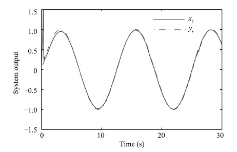
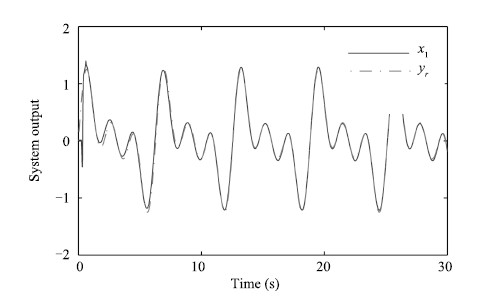
The design parameters for system (42) in the simulation study are chosen as $\Gamma _{\Psi 1} = 5I_{3 \times 3}$,$\Gamma _{\Psi 2} =0.5I_{4 \times 4}$,$\gamma _1 =500$,$\gamma _2$ $=$ $5$,$\chi _1 = \chi _2 = 10$,$K_1 =10$,$K_2 = 5$,$\mu_2=0.005$. The initial state conditions are arbitrarily chosen as $x_1 =x_2= 0$,the reference trajectory is taken as $y_r = \sin (0.5t)$. The design parameters for system (43) in the simulation study are chosen as $\Gamma _{\Psi 1} = 5I_{3 \times 3}$,$\Gamma _{\Psi 2} =0.5I_{4 \times 4}$,$\gamma _1 = 500$,$\gamma _2 = 5$,$\chi _1= \chi _2$ $=$ $5$,$K_1 = K_2 = 5$,$\mu_2=0.005$. The initial state conditions are arbitrarily chosen as $x_1 =0.01$,$x_2= 0$,the reference trajectory is taken as $y_r = 0.5*(\sin (t)+ \sin(2t)+ \sin(3t))$.
The tracking results of the uncertain non-affine system (42) and (43) are shown in

|
Download:
|
| Fig. 1. System output $y$ and reference signal $y_r$ for (42) | |

|
Download:
|
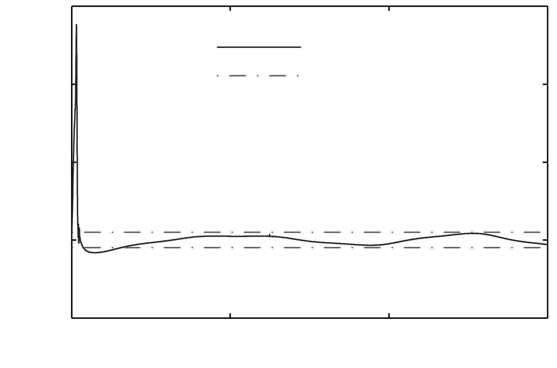
| Fig. 2. System tracking error for (42). | |

|
Download:
|
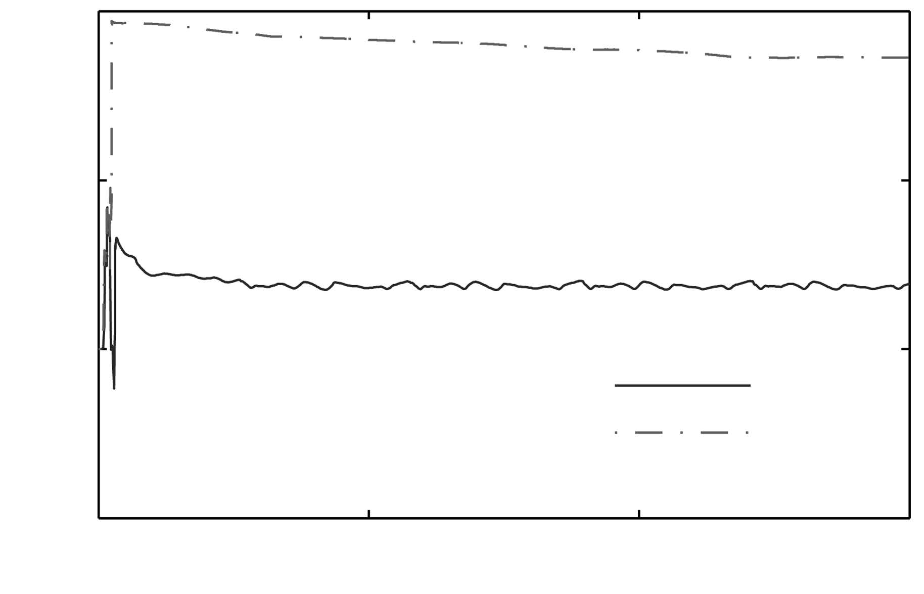
| Fig. 3. Adaptive parameters $\tau_1$ and $\tau_2 $ for (42). | |

|
Download:
|
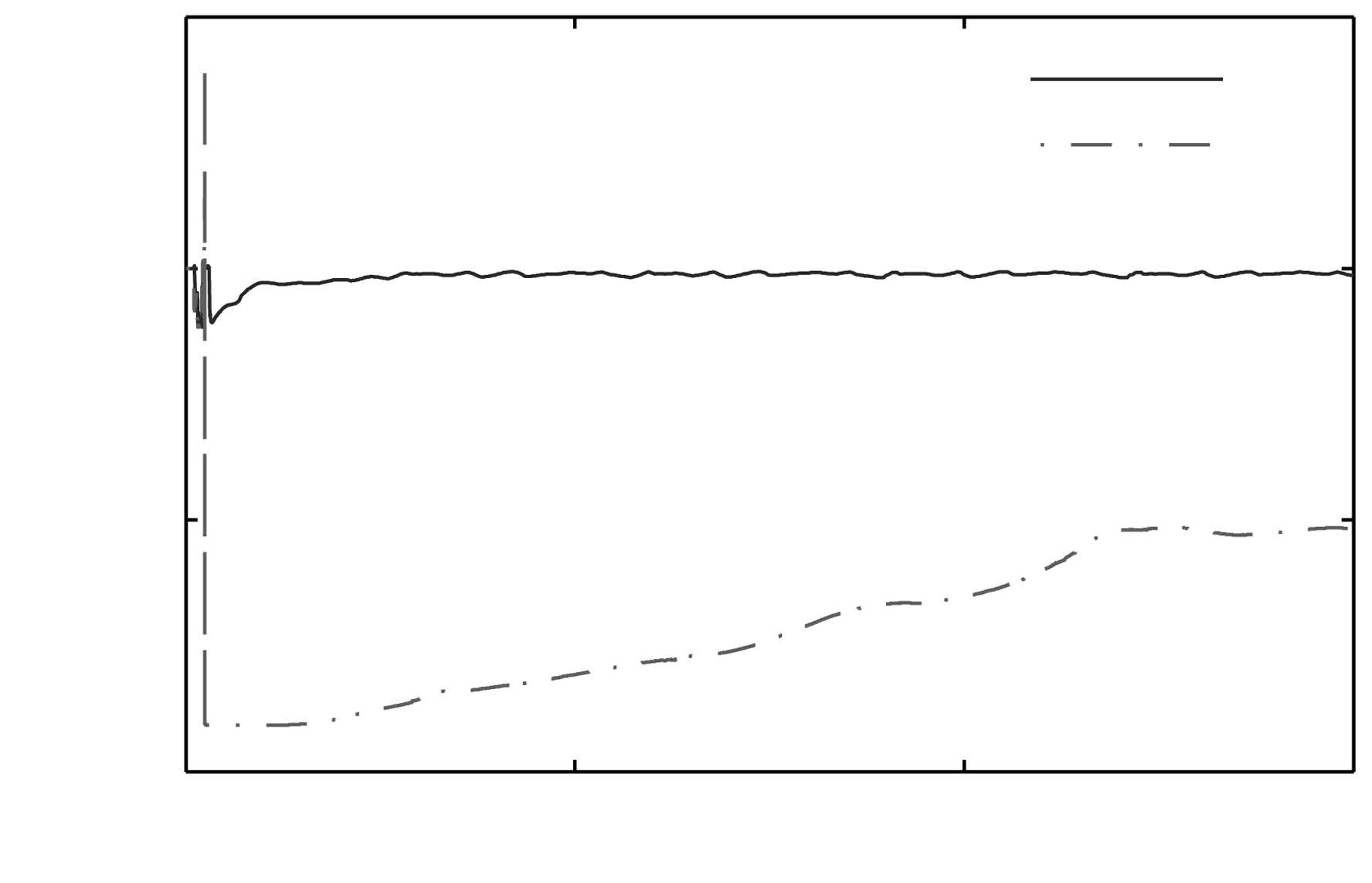
| Fig. 4. Nussbaum function $N ( \tau_1 )$ and $ N(\tau_2 )$ for (42). | |

|
Download:
|
| Fig. 5. System output $y$ and reference signal $y_r$ for (43). | |

|
Download:
|
| Fig. 6. System tracking error for (43). | |

|
Download:
|
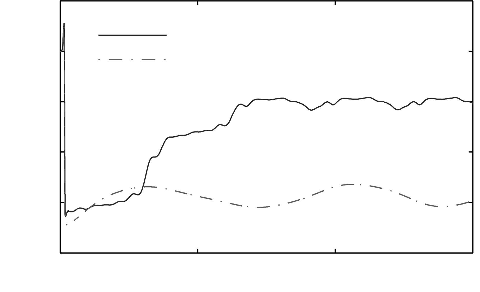
| Fig. 7. Adaptive parameters $\tau_1$ and $\tau_2 $ for (43). | |

|
Download:
|
| Fig. 8. Nussbaum function $N ( \tau_1 )$ and $ N(\tau_2 )$ for (43). | |
It is concluded from the simulation results that the proposed robust adaptive control technique for uncertain MIMO non-affine nonlinear systems is valid. In the process of controller design,it need not consider the structure and parameters of systems. If the systems have the same bound for each partial derivatives of the functions $f(\cdot)$,the structure of controllers is the same.
VI. CONCLUSIONAn adaptive robust tracking control has been proposed for a class of uncertain MIMO non-affine nonlinear systems in this paper. To improve the ability of the controller's robust performance,control singularity,disturbance attenuation,computation alleviation and real-time application,the mean value theorem has been employed to transform the non-affine system into affine-like form with strict feedback structure. Using adaptive algorithms with projection,DSC technique,nonlinear damping technique and Nussbaum gain technique,an adaptive robust tracking control has been proposed for MIMO non-affine nonlinear system with uncertain structure and parameters, unknown control direction and unknown external disturbance. The stability of the closed-loop system has been proved by Lyapunov analysis. Finally,simulation results have demonstrated the feasibility and validity of the proposed control schemes.
| [1] | Yeşidirek A, Lewis F L. Feedback linearization using neural networks. Automatica, 1995, 31(11):1659-1664 |
| [2] | Chen W S, Li J M. Adaptive output-feedback regulation for nonlinear delayed systems using neural network. International Journal of Automation and Computing, 2008, 5(1):103-108 |
| [3] | Li S Y, Xi Y G. A fuzzy-neural network control of nonlinear dynamic systems. Journal of Systems Engineering and Electronics, 2000, 11(1):61-66 |
| [4] | Li H X, Tong S C. A hybrid adaptive fuzzy control for a class of nonlinear MIMO systems. IEEE Transactions on Fuzzy Systems, 2003, 11(1):24-34 |
| [5] | Ge S S, Wang C. Adaptive neural control of uncertain MIMO nonlinear systems. IEEE Transactions on Neural Networks, 2004, 15(3):674-692 |
| [6] | Li Y H, Sheng Q, Zhang X Y, Kaynak O. Robust and adaptive backstepping control for nonlinear systems using RBF neural networks. IEEE Transactions on Neural Networks, 2004, 15(3):693-701 |
| [7] | Chen M, Ge S S, Ren B B. Adaptive tracking control of uncertain MIMO nonlinear systems with input constraints. Automatica, 2011, 47(3):452-465 |
| [8] | Zhang Y P, Peng P Y, Jiang Z P. Stable neural controller design for unknown nonlinear systems using backstepping. IEEE Transactions on Neural Networks, 2000, 11(6):1347-1360 |
| [9] | Huang S N, Tan K K, Lee T H. Nonlinear adaptive control of interconnected systems using neural networks. IEEE Transactions on Neural Networks, 2006, 17(1):243-246 |
| [10] | Krstić M, Kanellakopoulos I, Kokotović P V. Nonlinear and Adaptive Control Design. New York:Wiley, 1995. |
| [11] | Boskvoic J D, Chen L J, Mehra R K. Adaptive control design for nonaffine models arising in flight control. Journal of Guidance, Control, and Dynamics, 2004, 27(2):209-217 |
| [12] | Shiriaev A S, Ludvigsen H, Egeland O, Fradkov A L. Swinging up of non-affine in control pendulum. In:Proceedings of the 1999 American Control Conference. San Diego, California, USA:IEEE, 1999. 4039-4044 |
| [13] | Park J Y, Park G T. Robust adaptive fuzzy controller for non-affine nonlinear systems with dynamic rule activation. International Journal of Robust and Nonlinear Control, 2003, 13(2):117-139 |
| [14] | Labiod S, Guerra T M. Indirect adaptive fuzzy control for a class of nonaffine nonlinear systems with unknown control directions. International Journal of Control, Automation and Systems, 2010, 8(4):903-907 |
| [15] | Zhang Qiang, Wu Qing-Xian, Jiang Chang-Sheng, Wang Yu-Hui. Robust control for nonaffine nonlinear systems based on backstepping. Control and Decision, 2014, 29(1):19-26(in Chinese) |
| [16] | Arefi M M, Zarei J, Karimi H R. Adaptive output feedback neural network control of uncertain non-affine systems with unknown control direction. Journal of the Franklin Institute, 2014, 351(8):4302-4316 |
| [17] | Zhou Wei-Dong, Liao Cheng-Yi. Indirect adaptive fuzzy outputfeedback controller for a SISO nonaffine system with unknown control direction. Control Theory and Applications, 2013, 30(9):1131-1137(in Chinese) |
| [18] | Hu Yun-An, Li Hai-Yan. NN-based dynamic feedback backstepping control for nonaffine block nonlinear systems. Control and Decision, 2012, 27(1):65-70(in Chinese) |
| [19] | Gao D X, Sun Z Q, Liu J H. Dynamic inversion control for a class of pure-feedback systems. Asian Journal of Control, 2012, 14(2):605-611 |
| [20] | Zhao T. RBFN-based decentralized adaptive control of a class of largescale non-affine nonlinear systems. Neural Computing and Applications, 2008, 17(4):357-364 |
| [21] | Shen Q K, Shi P, Zhang T P, Lim C C. Novel neural control for a class of uncertain pure-feedback systems. IEEE Transactions on Neural Networks and Learning Systems, 2014, 25(4):718-727 |
| [22] | Ge S S, Wang C. Adaptive NN control of uncertain nonlinear purefeedback systems. Automatica, 2002, 38(4):671-682 |
| [23] | Sun G, Wang D, Li X Q, Peng Z H. A DSC approach to adaptive neural network tracking control for pure-feedback nonlinear systems. Applied Mathematics and Computation, 2013, 219(11):6224-6235 |
| [24] | Labiod S, Guerra T M. Adaptive fuzzy control of a class of SISO nonaffine nonlinear systems. Fuzzy Sets and Systems, 2007, 158(10):1126-1137 |
| [25] | Huang Y S, Zhou D Q, Chen X X. Decentralized direct adaptive output feedback fuzzy H∞ tracking design of large-scale nonaffine nonlinear systems. Nonlinear Dynamics, 2009, 58(1-2):153-167 |
| [26] | Lin W. Feedback stabilization of general nonlinear control systems:a passive system approach. Systems and Control Letters, 1995, 25(1):41-52 |
| [27] | Lin W. Global asymptotic stabilization of general nonlinear systems with stable free dynamics via passivity and bounded feedback. Automatica, 1996, 32(6):915-924 |
| [28] | Jia Tao, Liu Jun, Qian Fu-Cai. Adaptive fuzzy dynamic surface control for a class of nonlinear systems with unknown time-delays. Acta Automatica Sinica, 2011, 37(1):83-91(in Chinese) |
| [29] | Song M C, Lin Y. Robust adaptive output-feedback dynamic surface control of a class of nonlinear systems with unmodeled dynamics. Asian Journal of Control, 2013, 15(5):1337-1345 |
| [30] | Swaroop D, Hedrick J K, Yip P P, Gerdes J C. Dynamic surface control for a class of nonlinear systems. IEEE Transactions on Automatic Control, 2000, 45(10):1893-1899 |
| [31] | Song H T, Zhang T, Zhang G L, Lu C J. Robust dynamic surface control of nonlinear systems with prescribed performance. Nonlinear Dynamics, 2014, 76(1):599-608 |
| [32] | Ji G. Adaptive neural network dynamic surface control for perturbed nonlinear time-delay systems. International Journal of Automation and Computing, 2012, 9(2):135-141 |
| [33] | Boulkroune A, Tadjine M, Saad M M, Farza M. Fuzzy adaptive controller for MIMO nonlinear systems with known and unknown control direction. Fuzzy Sets and Systems, 2010, 161(6):797-820 |
| [34] | Wang J H, Hu J B. Robust adaptive control for uncertain nonlinear systems with unknown control directions and actuator nonlinearity. Journal of Control Theory and Applications, 2012, 10(4):441-450 |
| [35] | Ryan E P. A universal adaptive stabilizer for a class of nonlinear systems. Systems and Control Letters, 1991, 16(3):209-218 |
| [36] | Goodwin G C, Mayne D Q. A parameter estimation perspective of continuous time model reference adaptive control. Automatica, 1987, 23(1):57-70 |
| [37] | Zhou Li, Jiang Chang-Sheng. Improved robust and adaptive dynamic surface control for nonlinear systems. Control and Decision, 2008, 23(8):938-943(in Chinese) |