Ⅰ. Introduction

It is well known that nonlinear systems with asymptotically unstable zero dynamics or internal dynamics are called non-minimum phase^[1,2]. This feature cannot be removed by feedback,and restricts the straightforward application of the powerful nonlinear control techniques such as feedback linearization, sliding mode control and backstepping method^[3,4],which work well in minimum phase systems. Under this circumstance,the control problem of nonlinear non-minimum phase systems is more challenging and has been payed more attention by the control community.

The existing research work concerning the nonlinear non-minimum phase systems can be divided into two main branches: stabilization control and tracking control. Firstly we give a brief description on stabilization control for nonlinear non-minimum phase systems. Based on backstepping control and inverse design with the combination of neural network,^[5] implemented the state-feedback adaptive stabilization for a class of non-affine single-input single-output (SISO) non-minimum phase systems. Reference ^[6] achieved stabilization control for a class of nonlinear non-minimum phase systems in general output-feedback form via standard backstepping control and small-gain technique. In ^[7,8,9,10],different stabilization methods for non-minimum phase systems can be found, such as robust observer,neural network,and high-gain observer. Though the backstepping method cannot be directly used in non-minimum phase systems as described in ^[4],the aforementioned work properly introduced the backstepping into the stabilization control for those non-minimum phase systems under proper assumptions,and attained control aims. The common feature of these referred papers is that the outputs and the unstable internal dynamics are all stabilized to zero. As we all know,stabilization control is the basis of output tracking control,and output tracking can transformed into stabilization control problem of tracking errors^[3],so the aforesaid stabilization control methods can lead to the creation of output tracking control methods for nonlinear non-minimum phase systems.

Whereas the work such as ^[3,11,12] focus on another ambitious problem-trajectory tracking control of nonlinear non-minimum phase systems. When we design tracking control laws for minimum phase systems,the control aim is to let the system outputs to follow the desired output signals,and the internal dynamics are generally disregarded,because it will get stable when the external dynamics attains stability. However,this case is not applicable to non-minimum phase systems. For the tracking control of nonlinear non-minimum phase systems,the controller is designed to meet the following two demands: 1) The output tracking errors asymptotically converge to zero; 2) The unstable internal dynamics is rendered acceptable,that is,stabilized to zero^[13,14] or kept bounded^[15]. The output tracking problem of a nonlinear non-minimum phase VTOL aircraft was solved in ^[13] by a Lyapunov-based technique and a minimum-norm strategy. However,the internal dynamics which stands for the actual roll attitude of aircraft was directly stabilized to zero. In fact,this method is unfeasible for aircraft since it is impossible for its roll attitude to keep unchanged when it performs trajectory maneuver. Reference ^[15] pointed out that the proper method for presenting acceptable internal dynamics lies in finding a bounded solution for the unstable internal dynamics to follow,rather than directly stabilizing the internal dynamics to zero. The bound solution to the internal dynamics is originally called the ideal internal dynamics (IID) in ^[11,12] proposed noncausal stable inversion (NSI) method to construct the bounded IID for non-minimum phase systems. To obtain the causal IID for the unstable internal dynamics,^[3] originated the stable system center (SSC) method,which was used to solve the IID of non-minimum phase VTOL aircraft in ^[16]. The output regulation (OR) method in ^[17] can be used to find IID of non-minimum phase systems by solving partial differential algebraic equations.

As a survey on the control of nonlinear non-minimum phase systems, ^[18] discussed the features of three methods for the IID solution as follows: NSI is an iterative solution method,the desired trajectories and any of their changes must be exactly known in advance,the offline pre-computing procedure is conducted backward in time,thus it can only get numerical and noncausal solutions,so it is of limited practical use. Compared with NSI approach,SSC method does not necessarily require the future information of the desired trajectories which must be generated by an exosystem,the online solving procedure for bounded IID is performed forward in time,so the obtained numerical solutions are causal. OR method is applied to tackle the system with linear internal dynamics,and can provide accurate and analytical solutions.

Until now,there is few work about the output tracking control for nonlinear non-minimum phase systems in output-feedback form. This paper aims to solve this problem,and the contributions of this work can be summarized as follows:

1) To keep the unstable internal dynamics bounded,the method of output redefinition is introduced,thus the stability of the internal dynamics depends on that of the newly defined output. In the process of designing the control law,we only care about the external dynamics which includes the newly defined output,and disregard the internal dynamics,because it will get stable along with the stability of the external dynamics.

2) To overcome the explosion of complexity problem in traditional backstepping design,the dynamic surface control (DSC)^[19] method is firstly used to deal with the problem of tracking control for the nonlinear non-minimum phase systems in output-feedback form.

3) Benefiting from the bounded IID solved via SSC method,the paper realizes the casual output tracking for a class of nonlinear non-minimum phase systems.

The paper is organized as follows. In Section II,the class of controlled nonlinear non-minimum phase system in output-feedback form is introduced,and the control purpose is formulated. In Section III,the methods of observer-based output redefinition and the solution of IID are presented. In Section IV,the output feedback DSC design procedure is provided. Section V gives the stability analysis. In Section VI,a simulation example is given to show the effectiveness of the proposed design method. Section VII draws the conclusions.

Ⅱ. Problem Formulation

In the paper,we consider a class of nonlinear non-minimum phase systems in the following output-feedback form:

$\begin{align} & \dot{\eta }={{A}_{\eta }}\eta +{{B}_{\eta }}{{x}_{1}},\\ & {{{\dot{x}}}_{1}}={{x}_{2}}+{{\varphi }_{1}}(y),\\ & \qquad \qquad \vdots \\ & {{{\dot{x}}}_{n-1}}={{x}_{n}}+{{\varphi }_{n-1}}(y),\\ & {{{\dot{x}}}_{n}}={{E}_{\eta }}\eta +{{\varphi }_{n}}(y)+\beta (y)u,\\ & y={{x}_{1}},\\ \end{align}$

(1)

where $\eta \in {{R}^{m}}$ is internal dynamics; $(x_{1},...,x_{n})$ is the external dynamics; $u$ is the control input; $y$ is the output signal; Nonlinear items $\varphi _{i}(y)$ only depend on the output $y$,$i=1,$ $...,$ $n$. For all $y\in R $,the function $\beta (y)\neq 0$. We assume the matrix $A_{\eta }$ is non-Hurwitz,so when $x_{1}=0$, the corresponding zero dynamics $\dot{\eta}=A_{\eta }\eta $ is not asymptotically stable,thus $ \eta $ is the unstable internal dynamics,system (1) can be called non-minimum phase.

Since that the internal dynamics $\eta$ is unstable and only output $y$ is measured,the control object is to design an output feedback controller so that the system output $y$ can track the desired trajectory signal $y_{d}(t)$,while the unstable internal dynamics $\eta$ can follow its causal and bounded IID.

Ⅲ. Observe-based Output Redefinition A.Observer Design

Since only the output signal $y$ in (1) is available for measurement,a set of observers must be constructed to provide estimates of the unmeasured state variables $\eta,$ $x_{2},..., x_{n}$. To proceed,rewrite system (1) as

$\begin{align} &\dot{x} =Ax+\varphi (y)+b\beta (y)u,\\ &y =cx,\label{2.2} \end{align}$

(2)

in which

$\begin{align} & x={{\left[\begin{matrix} {{\eta }_{1\times m}},{{x}_{1}},...,{{x}_{n}} \\ \end{matrix} \right]}^{\text{T}}},\\ & \varphi (y)={{\left[\begin{matrix} {{\mathbf{0}}_{1\times m}},{{\varphi }_{1}}(y),...,{{\varphi }_{n}}(y) \\ \end{matrix} \right]}^{\text{T}}},\\ & A=\left[\begin{matrix} {{A}_{\eta }} & {{B}_{\eta }} & {{\mathbf{0}}_{m\times (n-1)}} \\ {{\mathbf{0}}_{(n-1)\times m}} & {{\mathbf{0}}_{(n-1)\times 1}} & {{I}_{n-1}} \\ {{E}_{\eta }} & 0 & {{\mathbf{0}}_{1\times (n-1)}} \\ \end{matrix} \right],\\ & b={{\left[\begin{matrix} {{\mathbf{0}}_{1\times m}} & {{\mathbf{0}}_{1\times (n-1)}} & 1 \\ \end{matrix} \right]}^{\text{T}}} \\ & c=\left[\begin{matrix} {{\mathbf{0}}_{1\times m}} & 1 & {{\mathbf{0}}_{1\times (n-1)}} \\ \end{matrix} \right],\\ \end{align}$

(3)

and $\mathbf{0}$,$I$ respectively stand for zero matrix and identity matrix.

By choosing vector $k$ such that $A_{0}=A-kc$ is a Hurwitz matrix,the following full-order observer is proposed for the purpose of the tracking control:

$\begin{align} &\dot{\hat{x}} =A\hat{x}+k(y-\hat{y})+\varphi (y)+b\beta (y)u,\\ &\hat{y}=c\hat{x}, \end{align}$

(4)

where the parameter $k=(k^{\rm T}_{\eta },k_{1},... ,k_{n})^{\rm T}$,and $k_{\eta }=(k_{\eta _{1}},$ $...,$ $k_{\eta _{m}})^{\rm T}.$ Subtracting (4) from (2),the observer error can be derived as

$\begin{align} \dot{\tilde{x}}=A_{0}\tilde{x},\label{2.4} \end{align}$

(5)

where $\tilde{x}=x-\hat{x}.$ Since $A_{0}$ is Hurwitz,the observer error $ \tilde{x}$ can exponentially converge to zero.

B.Output Redefinition

From (4),the observer equation of the internal dynamics can be written as

$\dot{\hat{\eta }}={{A}_{\eta }}\hat{\eta }+{{B}_{\eta }}{{\hat{x}}_{1}}+{{k}_{\eta }}{{\tilde{x}}_{1}}.$

(6)

To tackle the unstable internal dynamics $\hat{\eta}$,the new output is defined as

$\begin{align} \bar{x}_{1}=\hat{x}_{1}+M\hat{\eta},\label{2.6} \end{align}$

(7)

Thus (6) shows

$\dot{\hat{\eta }}={{A}_{\eta 0}}\hat{\eta }+{{B}_{\eta }}{{\bar{x}}_{1}}+{{k}_{\eta }}{{\tilde{x}}_{1}},$

(8)

where choosing $M$ to let $A_{\eta 0}=A_{\eta }-B_{\eta }M$ be Hurwitz. Since the observer error $\tilde{x}_{1}\rightarrow 0,$ the stability of internal dynamics $\hat{\eta}$ in (8) depends on the newly defined output $\bar{x}_{1}.$

After output redefinition,system (4) can be separated into the following two parts: new external dynamics

$\begin{gathered} \begin{array}{*{20}{c}} \cdot \\ {\bar x} \\ 1 \end{array} = {{\hat x}_2} + {\varphi _1}(y) + {k_1}{{\tilde x}_1} + M\mathop {\hat \eta }\limits^. {\mkern 1mu} , \hfill \\ \begin{array}{*{20}{c}} \cdot \\ {\hat x} \\ 2 \end{array} = {{\hat x}_3} + {\varphi _2}(y) + {k_2}{{\tilde x}_1}, \hfill \\ \vdots \hfill \\ \begin{array}{*{20}{c}} \cdot \\ {\hat x} \\ {n - 1} \end{array} = {{\hat x}_n} + {\varphi _{n - 1}}(y) + {k_{n - 1}}{{\tilde x}_1}, \hfill \\ \begin{array}{*{20}{c}} \cdot \\ {\hat x} \\ n \end{array} = {E_\eta }\hat \eta + {\varphi _n}(y) + {k_n}\tilde x{\ _1} + \beta (y)u, \hfill \\ \end{gathered} $

(9)

and the internal dynamics (8). Hereafter,we only design control law for the external dynamics $(\bar{x}_{1},\hat{x}_{2},... ,\hat{x}_{n})$ in (9),rather than the internal dynamics $\hat{\eta},$ because it will get stable with the stability of the external dynamics.

Remark 1. Note that the method of output redefinition originated from ^[11] is slightly revised in this paper,and the new output is based on the output observer system,rather than the original system.

C.Solution of IID

It is necessary to know the desired value of new output $\bar{x}_{1}$ before we design the output tracking control law. In (7),the desired value of output observer $\hat{x}_{1}$ is $y_{d}$, but what is the desired value of $\hat{\eta}$ ? In (6),$A_{\eta }$ is non-Hurwitz,so the internal dynamics does not have stable numerical solution. However,this does not mean that a bounded solution cannot be found for such an unstable system^[15]. In fact,under suitable assumptions,via NSI approach^[12] or the SSC method^[3], a bounded solution can be obtained. As to (6),setting $\hat{x} _{1}=y_{d},$ $\tilde{x}$ $=$ $0$,we can get a bounded solution of internal dynamics

$\begin{align} \dot{\eta}_{d}=A_{\eta }\eta _{d}+B_{\eta }y_{d},\label{2.10} \end{align}$

(10)

where $\eta _{d}$ is the so-called IID.

For the IID equation (10),we turn to the causal SSC method to solve $\eta _{d}.$ For convenience,(10) can be rewritten as

$\begin{align} \dot{\eta}_{d}=A_{\eta }\eta _{d}+\theta _{d}(y_{d}),\label{2.11} \end{align}$

(11)

where $\theta _{d}(y_{d})=B_{\eta }y_{d}$. We assume $\theta _{d}$ can be generated by a known exosystem

$\begin{align} \dot{w} =Sw,~~~ \theta _{d} =Cw. \label{2.12} \end{align}$

(12)

Its characteristic polynomial is

$\begin{array}{*{35}{l}} P(\lambda )= & \ \det (\lambda I-S) \\ = & \ {{\lambda }^{k}}+{{p}_{k-1}}{{\lambda }^{k-1}}+\cdots +{{p}_{1}}\lambda +{{p}_{0}}. \\ \end{array}$

(13)

Thus the causal IID $\eta _{d}$ can be solved by the following matrix differential equation

$\begin{align} \eta _{d}^{(k)}+&\ c_{k-1}\eta _{d}^{(k-1)}+\cdots +c_{1}\dot{\eta} _{d}+c_{0}\eta _{d} \\ =&\ -(P_{k-1}\theta _{d}^{(k-1)}+\cdots +P_{1}\theta _{d}+P_{0}\theta _{d}),\label{2.14} \end{align}$

(14)

where the parameters $c_{k-1},... ,c_{1},c_{0}$ depend on the desired eigenvalues,the matrix ${{P}_{k-1}},...,{{P}_{1}},{{P}_{0}}\in {{R}^{(n-r)\times (n-r)}}$ can be computed by the formula in ^[3].

Ⅳ. Control Law Design

In this section,we design control law for the external dynamics $(\bar{x}_{1},\hat{x}_{2},...,\hat{x}_{n})$ via dynamic surface method.

Step 1. Let the first error surface of new output be defined as

$\begin{align} S_{1}=\bar{x}_{1}-\bar{x}_{1d},\label{3.1} \end{align}$

(15)

where $\bar{x}_{1d}=y_{d}+M\eta _{d}.$ The time derivative of $S_{1}$ is

$\begin{align} \dot{S}_{1}=\dot{\bar{x}}_{1}-\dot{\bar{x}}_{1d}=\hat{x}_{2}+\varphi _{1}(y)+k_{1}\tilde{x}_{1}+M\dot{\hat{\eta}}-\dot{\bar{x}}_{1d}. \label{3.2} \end{align}$

(16)

Then a virtual control signal is selected as

$\begin{align} \hat{x}_{2d}=-l_{1}S_{1}-\varphi _{1}(y)-k_{1}\tilde{x}_{1}-M\dot{\hat{\eta}}% +\dot{\bar{x}}_{1d},\label{3.3} \end{align}$

(17)

and the error between $\hat{x}_{2}$ and $\hat{x}_{2d}$ is defined as

$\begin{align} \tilde{x}_{2d}=\hat{x}_{2}-\hat{x}_{2d}. \label{3.4} \end{align}$

(18)

$\begin{align} \dot{S}_{1}=-l_{1}S_{1}+\tilde{x}_{2d}. \label{3.5} \end{align}$

(19)

To avoid the explosion of terms in the process of computing $\dot{\hat{x}} _{2d}$,we let $\hat{x}_{2d}$ pass through a low-pass filter

$\begin{align} \tau _{2}\dot{\bar{x}}_{2d}+\bar{x}_{2d}=\hat{x}_{2d},~~~\bar{x}_{2d}(0)=\hat{x} _{2d}(0),\label{3.6} \end{align}$

(20)

where $\tau_{2}$ is a time constant. Thus $\bar{x}_{2d}$ is the filtered signal of $\hat{x}_{2d}$.

Step ${\pmb i}$ (2$\leq$ ${\pmb i}$ ${\bf \leq}$ ${\pmb n}$ ${\pmb -$} 1). Define the $i$-th error surface as

$\begin{align} S_{i}=\hat{x}_{i}-\bar{x}_{id},\label{3.7} \end{align}$

(21)

then the time derivative of $S_{i}$ satisfies

$\begin{align} \dot{S}_{i}=\dot{\hat{x}}_{i}-\dot{\bar{x}}_{id}=\hat{x}_{(i+1)}+\varphi _{i}(y)+k_{i}\tilde{x}_{1}-\dot{\bar{x}}_{id}. \label{3.8} \end{align}$

(22)

Choose a virtual control signal $\hat{x}_{(i+1)d}$ as

$\begin{align} \hat{x}_{(i+1)d}=-l_{i}S_{i}-\varphi _{i}(y)-k_{i}\tilde{x}_{1}+\dot{\bar{x}} _{id},\label{3.9} \end{align}$

(23)

and define the error between $\hat{x}_{i+1}$ and $\hat{x}_{(i+1)d}$ as

$\begin{align} \tilde{x}_{(i+1)d}=\hat{x}_{i+1}-\hat{x}_{(i+1)d}. \label{3.10} \end{align}$

(24)

Thus we can get

$\begin{align} \dot{S}_{i}=-l_{i}S_{i}+\tilde{x}_{(i+1)d}. \label{3.11} \end{align}$

(25)

Letting $\bar{x}_{(i+1)d}$ be the filtered signal of $\hat{x}_{(i+1)d}$,that is,

$\begin{align} & {{\tau }_{i+1}}{{{\dot{\bar{x}}}}_{(i+1)d}}+{{{\bar{x}}}_{(i+1)d}}={{{\hat{x}}}_{(i+1)d}},\\ & {{{\bar{x}}}_{(i+1)d}}(0)={{{\hat{x}}}_{(i+1)d}}(0),\\ \end{align}$

(26)

where $\tau _{i+1}$ is a positive time constant.

Step ${\pmb n$.} Finally,define the $n$-th error surface as

$\begin{align} S_{n}=\hat{x}_{n}-\bar{x}_{nd},\label{3.13} \end{align}$

(27)

thus

$\begin{array}{*{35}{l}} {{{\dot{S}}}_{n}} & ={{{\dot{\hat{x}}}}_{n}}-{{{\dot{\bar{x}}}}_{nd}} \\ {} & ={{E}_{\eta }}\hat{\eta }+{{\varphi }_{n}}(y)+{{k}_{n}}{{{\tilde{x}}}_{1}}+\beta (y)u-{{\overset{.}{\mathop{{\bar{x}}}}\,}_{nd}}. \\ \end{array}$

(28)

The actual control signal is thus chosen as

$u=\frac{-{{l}_{n}}{{S}_{n}}-{{E}_{\eta }}\hat{\eta }-{{\varphi }_{n}}(y)-{{k}_{n}}{{{\tilde{x}}}_{1}}+{{\overset{.}{\mathop{{\bar{x}}}}\,}_{nd}}}{\beta (y)}.$

(29)

It could be readily checked that

$\begin{align} \dot{S}_{n}=-l_{n}S_{n}. \label{3.16} \end{align}$

(30)

Remark 2. According to the conventional backstepping method^[4,20],the actual control signal shows

$\begin{align} u=\frac{1}{\beta (y)}\left(\alpha _{n}-E_{\eta }\hat{\eta}+\bar{x}_{1d}^{(n)}\right),\label{2.33} \end{align}$

(31)

where

$\begin{array}{*{35}{l}} {{\alpha }_{n}}= & -{{l}_{n}}{{S}_{n}}-{{S}_{n-1}}-{{d}_{n}}{{\left( \frac{\partial {{\alpha }_{n-1}}}{\partial y} \right)}^{2}}{{S}_{i}}-{{k}_{i}}{{{\tilde{x}}}_{1}} \\ {} & -\frac{\partial {{\alpha }_{n-1}}}{\partial y}({{{\hat{x}}}_{2}}+{{\varphi }_{1}}(y)) \\ {} & -\sum\limits_{j=1}^{n-1}{\frac{\partial {{\alpha }_{n-1}}}{\partial {{{\hat{x}}}_{j}}}}({{\widehat{x}}_{j+1}}+{{\varphi }_{1}}(y)+{{k}_{j}}{{{\tilde{x}}}_{1}}) \\ {} & -\sum\limits_{j=1}^{m}{\frac{\partial {{\alpha }_{n-1}}}{\partial {{{\hat{\eta }}}_{j}}}}{{{\dot{\hat{\eta }}}}_{j}}-\sum\limits_{j=1}^{n-2}{\frac{\partial {{\alpha }_{n-1}}}{\partial \bar{x}_{1d}^{(j)}}}\bar{x}_{1d}^{(j+1)},\\ {{S}_{n}}= & \ {{{\hat{x}}}_{n}}-{{\alpha }_{n-1}}-\bar{x}_{1d}^{(n-1)},\\ {{\alpha }_{1}}= & -{{l}_{1}}{{S}_{1}}-{{d}_{1}}{{({{k}_{1}}+M{{k}_{\eta }})}^{2}}{{S}_{1}} \\ {} & -{{\varphi }_{1}}(y)-M{{A}_{\eta }}\hat{\eta }-M{{B}_{\eta }}{{{\hat{x}}}_{1}},\\ {{S}_{1}}= & \ {{{\bar{x}}}_{1}}-{{{\bar{x}}}_{1d}},\\ \end{array}$

(32-35)

and $S_{i},\alpha_{i}$ $(i=2,...,n-1)$ have similar forms as $S_{n},\alpha_{n}$.

Obviously,compared with the backstepping method,the proposed DSC scheme is simpler,and is easier to be realized in the practical systems with the increase of the dimension $m$ of internal dynamics and system relative order $n$.

Ⅴ. Stability Analysis

In this section,we will give the stability analysis for the proposed output-feedback DSC scheme. While the control law design procedure is simple,the stability analysis is relatively complicated due to the derivation of low-pass filter. Firstly, define the filter error as

$\begin{align} z_{i}=\hat{x}_{id}-\bar{x}_{id},~~~i=2,... ,n. \label{3.17} \end{align}$

(36)

Taking (26) into consideration,the time derivative of $ \bar{x}_{id}$ shows

$\begin{align} \dot{\bar{x}}_{id}=\frac{1}{\tau _{i}}(\hat{x}_{id}-\bar{x}_{id})=\frac{1}{ \tau _{i}}z_{i}. \label{3.18} \end{align}$

(37)

Thus

$\begin{align} \dot{z}_{i}=\dot{\hat{x}}_{id}-\dot{\bar{x}}_{id}=-\frac{1}{\tau _{i}}z_{i}+ \dot{\hat{x}}_{id}. \label{3.19} \end{align}$

(38)

By considering (21) and (36),$\tilde{x}_{id}$ in (24) can be rewritten as

$\begin{align} \tilde{x}_{id}& =\hat{x}_{i}-\hat{x}_{id}\\ & =\hat{x}_{i}-\bar{x}_{id}+\bar{x}_{id}-\hat{x}_{id}\\ & =S_{i}-z_{i}. \label{3.20} \end{align}$

(39)

So the error surface in (19) and (25) can be described as

$\begin{align} \dot{S}_{i}=-l_{i}S_{i}+S_{i+1}-z_{i+1},\quad i=1,...,n-1. \end{align}$

(40)

On the other side,from (5)-(17),(21)-(23),we can obtain

$\begin{align} \dot{z}_{i}& +\frac{1}{\tau _{i}}z_{i} \\ & =\dot{\hat{x}}_{id} \leq B_{i}(S_{i-1},S_{i},z_{i},\tilde{x},\bar{x}_{(i-1)d},\dot{\bar{x}}_{(i-1)d},\ddot{\bar{x}}_{(i-1)d}),\\ &\qquad\qquad\qquad\qquad\qquad\qquad\qquad\qquad\ \ i=2,...,n, \label{3.22} \end{align}$

(41)

where $B_{i},$ $i=2,...,n,$ are continuous positive functions. Thus

$\begin{align} z_{i}\dot{z}_{i} &\leq -\frac{1}{\tau _{i}}z_{i}^{2}+B_{i}\left\vert z_{i}\right\vert \\[1mm] & \leq \left(\frac{B_{i}^{2}}{2\alpha _{i}}-\frac{1}{\tau _{i}}\right)z_{i}^{2}+\frac{1 }{2}\alpha _{i},\quad i=2,...,n,\label{3.23} \end{align}$

(42)

where $\alpha _{i}$ are positive constants.

Secondly,define the tracking error of internal dynamics as

$\begin{align} \tilde{\eta}=\hat{\eta}-\eta _{d}. \label{3.24.1} \end{align}$

(43)

According to (8),(10) and (15),we can get

$\dot{\tilde{\eta }}={{A}_{\eta 0}}\tilde{\eta }+{{B}_{\eta }}{{S}_{1}}+{{k}_{\eta }}\tilde{x}$

(44)

By considering the aforementioned equations,the resulting closed-loop system can be expressed as

$\dot{\tilde{x}}={{A}_{0}}\tilde{x},$

(45)

$\dot{\tilde{\eta }}={{A}_{\eta 0}}\tilde{\eta }+{{B}_{\eta }}{{S}_{1}}+{{k}_{\eta }}{{\widetilde{x}}_{1}},$

(46)

${{{\dot{S}}}_{i}}=-{{l}_{i}}{{S}_{i}}+{{S}_{i+1}}-{{z}_{i+1}},\quad i=1,...,n-1,$

(47)

${{{\dot{S}}}_{n}}=-{{l}_{n}}{{S}_{n}},$

(48)

${{z}_{i}}{{\dot{z}}_{i}}\le \left( \frac{B_{i}^{2}}{2{{\alpha }_{i}}}-\frac{1}{{{\tau }_{i}}} \right)z_{i}^{2}+\frac{1}{2}{{\alpha }_{i}},\quad i=2,...,n.$

(49)

Next,we present the following theorem.

Theorem 1. Consider the Lyapunov function candidate as

$\begin{align} V=\sum_{i=0}^{n}V_{i},\label{3.30} \end{align}$

(50)

where

${{V}_{0}}={{{\tilde{\eta }}}^{\text{T}}}{{P}_{\eta }}\tilde{\eta }+{{{\tilde{x}}}^{\text{T}}}{{P}_{0}}\tilde{x},$

(51)

${{V}_{i}}=\frac{1}{2}S_{i}^{2}+\frac{{{d}_{i}}}{2}z_{i+1}^{2},\quad 1\le i\le n-1,$

(52)

${{V}_{n}}=\frac{1}{2}S_{n}^{2},$

(53)

and $P_{\eta }=P_{\eta }^{\rm T},P_{0}=P_{0}^{\rm T}$ respectively stand for the symmetric positive solutions of $P_{\eta }A_{\eta 0}+A_{\eta 0}^{\rm T}P_{\eta }=-I$,$P_{0}A_{0}+A_{0}^{\rm T}P_{0}$ $=$ $-I$,$A_{\eta 0}$ is defined by (8). For the given compact set $\Omega $,if

$\begin{align} V(0)=\sum_{i=0}^{n}V_{i}(0)\leq R_{0},\label{3.34} \end{align}$

(54)

then there exist $\gamma,$ $r$,$l_{i}$ $(i=1,...,n),$ $d_{i}$ $(i=1,...,n-1),$ and $\tau _{i}$ $ (i=2,...,n)$ to let all signals of the closed-loop system be bounded,the tracking errors can converge to some residual sets that can be made arbitrarily small by properly choosing certain design parameters.

Proof. The time derivative of $V_{0}$ is

$\begin{array}{*{35}{l}} {{{\dot{V}}}_{0}}= & \ {{{\tilde{\eta }}}^{\text{T}}}A_{\eta 0}^{\text{T}}{{P}_{\eta }}\tilde{\eta }+{{\eta }^{\text{T}}}{{P}_{\eta }}{{A}_{\eta 0}}\tilde{\eta }+{{S}_{1}}B_{\eta }^{\text{T}}{{P}_{\eta }}\eta \\ {} & +{{{\tilde{\eta }}}^{\text{T}}}{{P}_{\eta }}{{B}_{\eta }}{{S}_{1}}+{{{\tilde{x}}}_{1}}k_{\eta }^{\text{T}}{{P}_{\eta }}\tilde{\eta }+{{{\tilde{\eta }}}^{\text{T}}}{{P}_{\eta }}{{k}_{\eta }}{{{\tilde{x}}}_{1}} \\ {} & +{{{\tilde{x}}}^{\text{T}}}A_{0}^{\text{T}}{{P}_{0}}\tilde{x}+{{{\tilde{x}}}^{\text{T}}}{{P}_{0}}{{A}_{0}}\tilde{x} \\ = & -{{{\tilde{\eta }}}^{\text{T}}}\hat{\eta }+\gamma S_{1}^{2}+\frac{1}{\gamma }{{{\tilde{\eta }}}^{\text{T}}}(P_{\eta }^{\text{T}}{{B}_{\eta }}B_{\eta }^{\text{T}}{{P}_{\eta }})\tilde{\eta } \\ {} & +\gamma \tilde{x}_{1}^{2}+\frac{1}{\gamma }{{{\tilde{\eta }}}^{\text{T}}}(P_{\eta }^{\text{T}}{{k}_{\eta }}k_{\eta }^{\text{T}}{{P}_{\eta }})\tilde{\eta }-{{{\tilde{x}}}^{\text{T}}}\tilde{x} \\ \le & -\left( \frac{1}{{{\lambda }_{\max }}({{P}_{\eta }})}-\frac{{{\lambda }_{\max }}(P_{\eta }^{\text{T}}{{B}_{\eta }}B_{\eta }^{\text{T}}P)}{\gamma {{\lambda }_{\min }}({{P}_{\eta }})} \right. \\ {} & amp;\left. -\frac{{{\lambda }_{\max }}(P_{\eta }^{\text{T}}{{k}_{\eta }}k_{\eta }^{\text{T}}{{P}_{\eta }})}{\gamma {{\lambda }_{\min }}({{P}_{\eta }})} \right){{{\tilde{\eta }}}^{\text{T}}}{{P}_{\eta }}\tilde{\eta } \\ {} & amp;+\gamma S_{1}^{2}-\left( \frac{1}{{{\lambda }_{\max }}({{P}_{0}})}-\frac{\gamma }{{{\lambda }_{\min }}({{P}_{0}})} \right){{{\tilde{x}}}^{\text{T}}}{{P}_{0}}\tilde{x}. \\ \end{array}$

(55)

The derivative of $V_{i}$ satisfies

$\begin{array}{*{35}{l}} {{{\dot{V}}}_{i}}= & \ {{S}_{i}}(-{{l}_{i}}{{S}_{i}}+{{S}_{i+1}}-{{z}_{i+1}})+{{d}_{i}}{{z}_{i+1}}{{{\dot{z}}}_{i+1}} \\ \le & -{{l}_{i}}S_{i}^{2}+S_{i}^{2}+\frac{1}{2{{d}_{i}}}S_{i+1}^{2}+\frac{{{d}_{i}}}{2}z_{i+1}^{2} \\ {} & +{{d}_{i}}\left( \frac{B_{i+1}^{2}}{2{{\alpha }_{i+1}}}-\frac{1}{{{\tau }_{i+1}}} \right)z_{i+1}^{2}+\frac{{{d}_{i}}}{2}{{\alpha }_{i+1}} \\ \le & -({{l}_{i}}-1)S_{i}^{2}+\frac{1}{2{{d}_{i}}}S_{i+1}^{2} \\ {} & -{{d}_{i}}\left( \frac{1}{{{\tau }_{i+1}}}-\frac{B_{i+1}^{2}}{2{{\alpha }_{i+1}}}-\frac{1}{2} \right)z_{i+1}^{2}+\frac{{{d}_{i}}}{2}{{\alpha }_{i+1}}. \\ \end{array}$

(56)

Define the compact set as

$\begin{align} \Omega =&\ \bigg\{(S_{1},...,S_{n},z_{2},...,z_{n},\tilde{x},\eta_{d},\bar{x} _{1d},...,\bar{x}_{(n-1)d},\\ &\quad\ \dot{\bar{x}}_{1d},... ,\dot{\bar{x}}_{(n-1)d},\ddot{\bar{x}}_{1d},... ,\ddot{\bar{x}}_{(n-1)d}) : \\ &\quad \sum_{i=1}^{n}S_{i}^{2}+\sum_{i=2}^{n}z_{i}^{2}+\tilde{x}^{\rm T}\tilde{x} +\eta _{d}^{\rm T}\eta _{d}+\sum_{i=2}^{n}\bar{x}_{(i-1)d}^{2} \\ &\quad +\sum_{i=2}^{n}\dot{\bar{x}} _{(i-1)d}^{2}+\sum_{i=2}^{n}\ddot{\bar{x}}_{(i-1)d}^{2} \leq R_{0}\bigg\}, \end{align}$

(57)

where $R_{0}$ is a positive constant. Since $B_{i+1}$ defined by (41) is continuous,it has a maximum value in $\Omega $,i.e., $M_{i+1}$. So the derivative of $V_{i}$ shows

$\begin{array}{*{35}{l}} {{{\dot{V}}}_{i}}\le & -({{l}_{i}}-1)S_{i}^{2}+\frac{1}{2{{d}_{i}}}S_{i+1}^{2} \\ {} & -{{d}_{i}}\left( \frac{1}{{{\tau }_{i+1}}}-\frac{M_{i+1}^{2}}{2{{\alpha }_{i+1}}}-\frac{1}{2} \right)z_{i+1}^{2}+\frac{{{d}_{i}}}{2}{{\alpha }_{i+1}}. \\ \end{array}$

(58)

Finally,in view of (30),the derivative of $V_{n}$ yields

$\begin{align} \dot{V}_{n}=S_{n}\dot{S}_{n}=-l_{n}S_{n}^{2}. \label{3.38} \end{align}$

(59)

So

$\begin{align} \dot{V} \leq& -\left(\frac{1}{\lambda _{\max }(P_{\eta })}-\frac{\lambda _{\max }(P_{\eta }^{\rm T}B_{\eta }B_{\eta }^{\rm T}P)}{\gamma \lambda _{\min }(P_{\eta })}\right. \\ & \left.-\frac{\lambda _{\max }(P_{\eta }^{\rm T}k_{0}k_{0}^{\rm T}P_{\eta })}{\gamma \lambda _{\min }(P_{\eta })}\right)\hat{\eta}^{\rm T}P_{\eta }\hat{\eta} \\ & -\left(\frac{1}{\lambda_{\max}(P_{0})}-\frac{\gamma}{\lambda_{\min}(P_{0})}\right)\tilde{x}^{\rm T}P_{0}\tilde{x} \\ & +\frac{1}{2}\sum_{i=1}^{n-1}d_{i}\alpha _{i+1}-\sum_{i=1}^{n-1}\left(c_{i}-\frac{ 1}{2d_{i}}-1-\gamma\right)S_{i}^{2} \\ & -\sum_{i=1}^{n-1}\left(\frac{1}{\tau _{i+1}}-\frac{M_{i+1}^{2}}{2\alpha _{i+1}}- \frac{1}{2}\right)d_{i}z_{i+1}^{2} \\ & +\left(l_{n}-\frac{1}{2}\right)S_{n}^{2}. \end{align}$

(60)

Then let the design parameters

$\begin{align} & \frac{1}{{{\lambda }_{\max }}({{P}_{\eta }})} \\ & \ \quad =2r+\frac{{{\lambda }_{\max }}(P_{\eta }^{\text{T}}{{B}_{\eta }}B_{\eta }^{\text{T}}P)}{\gamma {{\lambda }_{\min }}({{P}_{\eta }})}\times \frac{{{\lambda }_{\max }}(P_{\eta }^{\text{T}}{{k}_{\eta }}k_{\eta }^{\text{T}}{{P}_{\eta }})%}{\gamma {{\lambda }_{\min }}({{P}_{\eta }})},\\ \end{align}$

(61)

$\frac{1}{{{\lambda }_{\max }}({{P}_{0}})}=2r+\frac{\gamma }{{{\lambda }_{\min }}({{P}_{0}})},$

(62)

${{l}_{i}}=r+\frac{1}{2{{d}_{i}}}+1+\gamma ,$

(63)

$\frac{1}{{{\tau }_{i+1}}}=r+\frac{M_{i+1}^{2}}{2{{\alpha }_{i+1}}}+\frac{1}{2},$

(64)

${{l}_{n}}=r+\frac{1}{2},$

(65)

where $r$ is a positive constant,it follows that

$\begin{align} \dot{V}\leq -2rV+M,\label{3.41} \end{align}$

(66)

where

$\begin{align} M=\frac{1}{2}\sum_{i=1}^{n-1}d_{i}\alpha _{i}. \label{3.42} \end{align}$

(67)

So when $V=R_{0}$,we have $\dot{V}\leq -2rR_{0}+M$. That is,if $r$ is chosen such that

$\begin{align} r>\frac{M}{2R_{0}}, \end{align}$

(68)

we have $\dot{V}<0$ on $V=R_{0}$,which implies that if $V(0)\leq R_{0}$,then $V(t)\leq R_{0}$ for all $t\geq 0$,i.e.,$V\leq R_{0}$ is an invariant set. Moreover,solving (66) yields

$\begin{align} 0\leq V\leq \frac{M}{2r}+\left(V(0)-\frac{M}{2r}\right){\rm e}^{-2rt}. \end{align}$

(69)

Hence

$\begin{align} \mathop{{\lim }}_{{\rm T}\rightarrow {0}}V(t)\leq \frac{M}{2r}. \end{align}$

(70)

That is,by properly choosing $\gamma ,$ $l_{i}$ $(i=1,... ,n),$ $d_{i}$ $(i=1,$ $...,$ $n-1),$ $\tau _{i}$ $(i=2,...,n)$ to make $M$ sufficiently small,$r$ sufficiently large,the tracking error $S_{i}$ $(i=1,...,n)$ can converge to any arbitrary small residual set. Since the observer error $ \tilde{x}$ exponentially converges to zero,and the desired output signal $ y_{d}$ and the IID $\eta _{d}$ are all bounded,so all the signals of the closed-loop system are uniformly bounded.

Ⅵ. Simulation Results

We consider the following nonlinear non-minimum phase system:

$\begin{align} &\dot{x}_{1} =x_{2}+\sin y,\\ &\dot{x}_{2} =x_{3}+y,\\ &\dot{x}_{3} =\eta+100(y^{2}+1)u,\\ &\dot{\eta} =\eta+x_{1},\\ &y =x_{1},\label{3.46} \end{align}$

(71)

where $\eta$ is the unstable internal dynamics. The goal is to apply the proposed output-feedback DSC scheme to (71) so that the system output $y$ and the internal dynamics $\eta$ can respectively track their desired signals $y_{d}$ and $\eta_{d}$.

A.IID Solution via SSC Method

At the beginning of the simulation,we firstly need to solve the IID $\eta _{d}$ of system (71) according to the SSC method described as (11)-(14). As to the internal dynamics equation $\dot{\eta}$ $=$ $\eta+x_{1}$,by setting $x_{1}=y_{d}$,its corresponding IID equation shows

$\begin{align} \dot{\eta}_{d}=\eta _{d}+y_{d}. \label{3.46.1} \end{align}$

(72)

By selecting the desired trajectory signal $y_{d}=R\cos (\omega t)$,it can be generated by the following exosystem

$\begin{align} & \dot{w}=Sw,\\ & S=\left( \begin{matrix} 0 & \omega \\ -\omega & 0 \\ \end{matrix} \right),\\ \end{align}$

(73)

whose characteristic polynomial is

$\begin{align} P(\lambda )=\left\vert \lambda I-S\right\vert =\lambda ^{2}+\omega ^{2}. \label{2.58} \end{align}$

(74)

According to the above equation,we can get $k=2$,$p_{1}=0$ and $p_{0}=\omega ^{2}.$ By setting the desired eigenvalues $s_{1,2}=-1,$ thus the parameters of the characteristic polynomial are $c_{0}=$ $1,$ $c_{1}=2$. Via the SSC method in 3,we can get

$\begin{align} & {{P}_{1}}=(I+2Q_{1}^{-1}+Q_{1}^{-2}){{(I+{{\omega }^{2}}Q_{1}^{-2})}^{-1}}-I=\frac{3-{{\omega }^{2}}}{1+{{\omega }^{2}}},\\ & {{P}_{0}}={{c}_{0}}Q_{1}^{-1}-({{P}_{1}}+I){{p}_{0}}Q_{1}^{-1}=\frac{1-3{{\omega }^{2}}}{1+{{\omega }^{2}}},\\ \end{align}$

(75)

where $Q_{1}=A_{\eta }=1$. By taking the parameters $c_{0},$ $c_{1},$ $ P_{1}$ and $P_{0}$ into the matrix differential equation (14),the IID $\eta_{d}$ can be solved from the following equation:

$\begin{align} \ddot{\eta}_{d}+c_{1}\dot{\eta}_{d}+c_{0}\eta _{d}=-(P_{1}\dot{\theta} _{d}+P_{0}\theta _{d}). \label{3.49} \end{align}$

(76)

B.IID Comparison

Here through the IID equation (72),we give a detailed comparison of IID solved via the aforementioned methods: NSI,SSC,OR. Through OR method,the accurate and analytical bounded solution is

$\begin{align} \eta_{d}=\frac{R\omega ^{2}\cos(\omega t)+R\omega\sin(\omega t)}{1+\omega ^{2}}. \end{align}$

(77)

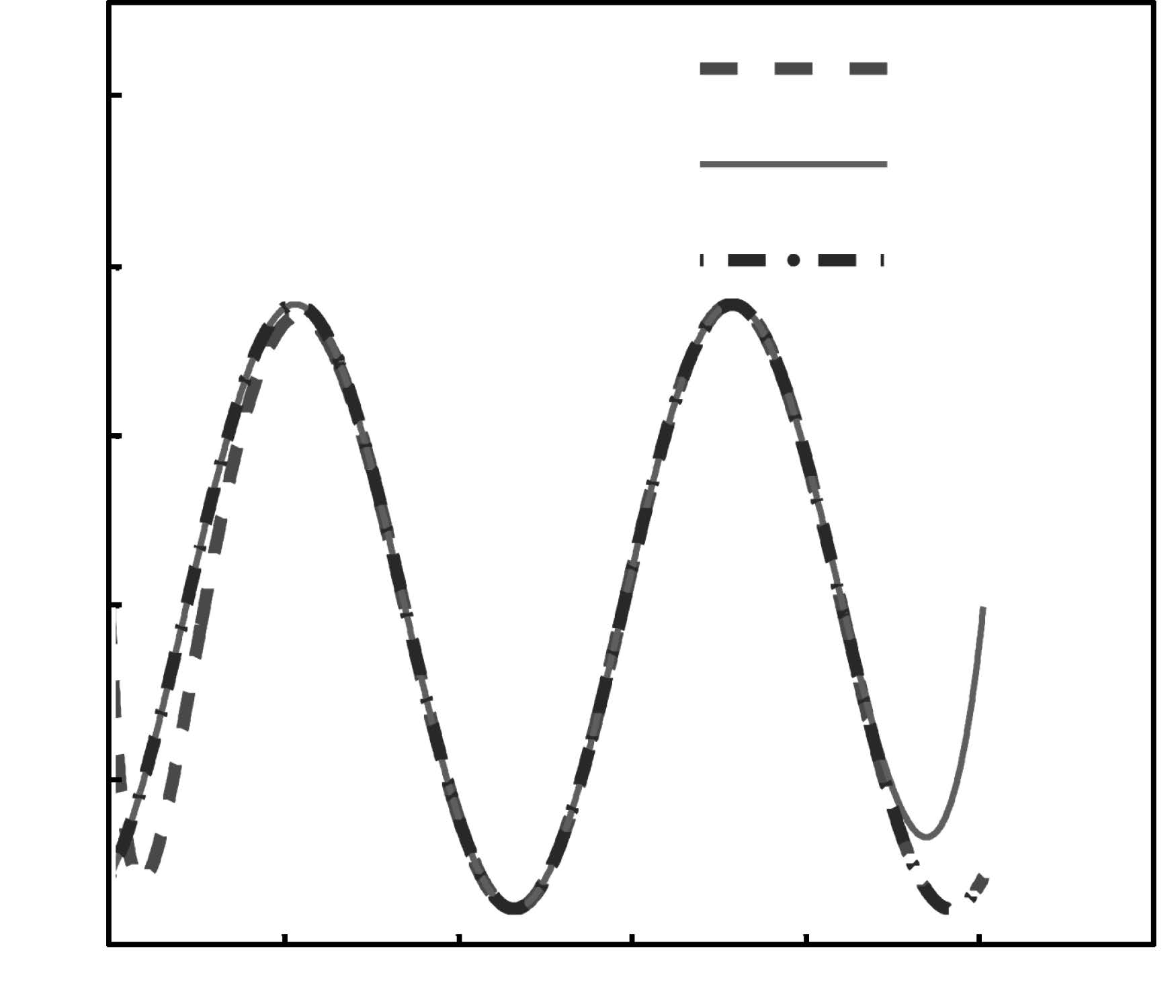
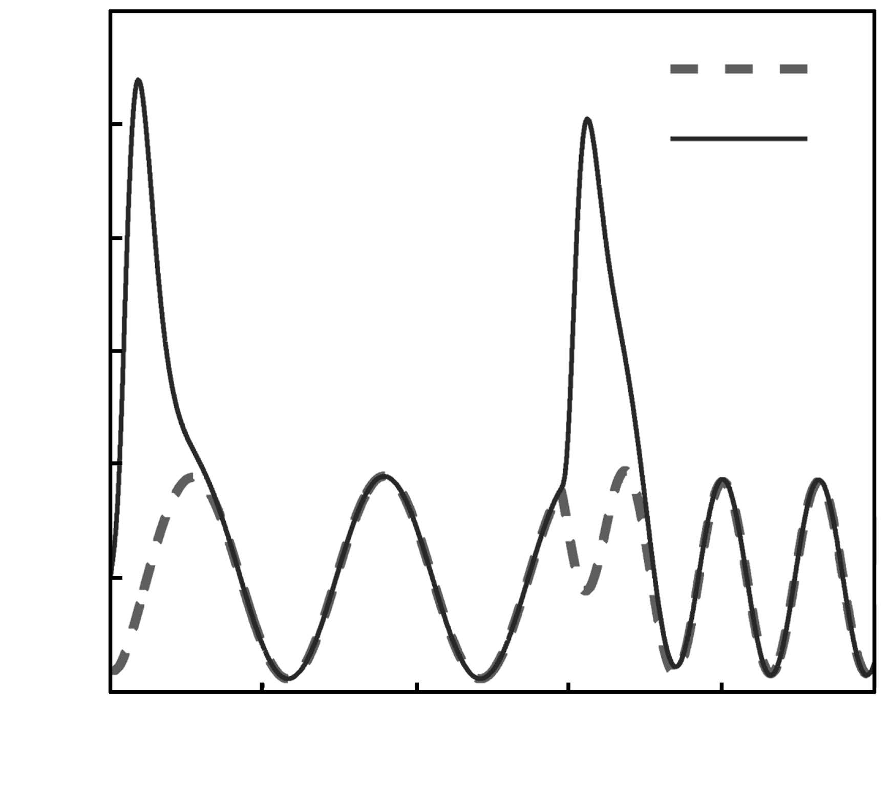
Detailed solution procedure of NSI and OR methods can be found in 17. By selecting $R=1$,$\omega=1$,the solved IID $\eta _{d}$ of the system (71) can be seen in Fig.1.

From Fig.1,it can be seen that the IID solved via SSC method gradually converge to the accurate and analytical IID solved via OR method,while the IID solved NSI method would diverge from the IID solved via OR method at the end of simulation time,because the off-line pre-computing procedure of NSI method is conducted backward in time. Due to the limited practical use of NSI method, we turn to the SSC method to get the causal IID of (71).

C.Simulation Results

The system initial states are selected as $x(0)=(0.95,$ $0,$ $0,$ $0)^{\rm T}$,$\hat{x}(0)=(1,0,0,0)^{\rm T}$,$\eta_{d}(0)=-0.8$; The observer gain is selected as $k=(13,67,175,257)^{\rm T}$ to let the eigenvalues of $A_{0}$ be $-3$. The controller parameters $l_{1}=l_{2}=l_{3}=15$,the filter time constant $\tau _{2}=\tau_{3}=0.01$. The output transformation matrix is chosen as $M=2$ to place the eigenvalues of $A_{\eta 0}$ at $-1$. The desired output signal is selected as $y_{d}=R\cos(\omega t)$. To illustrate the effectiveness of the proposed control scheme,the simulations are done under the following two cases.

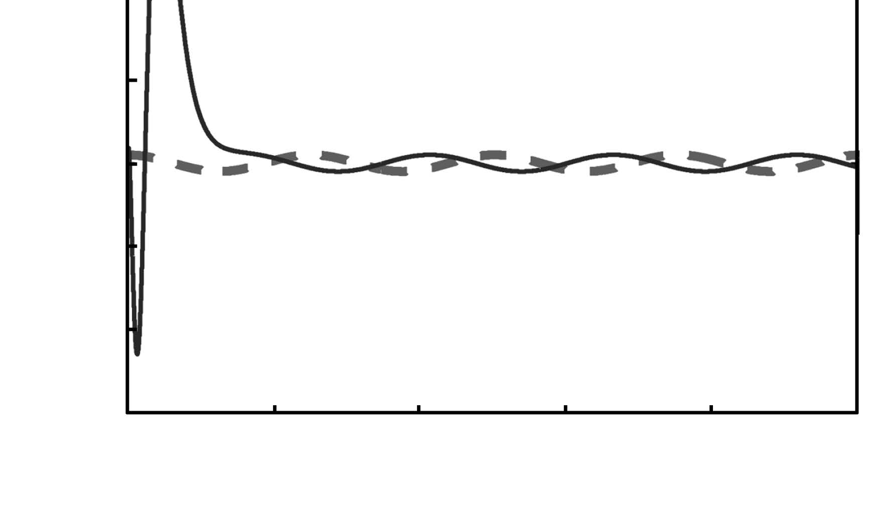
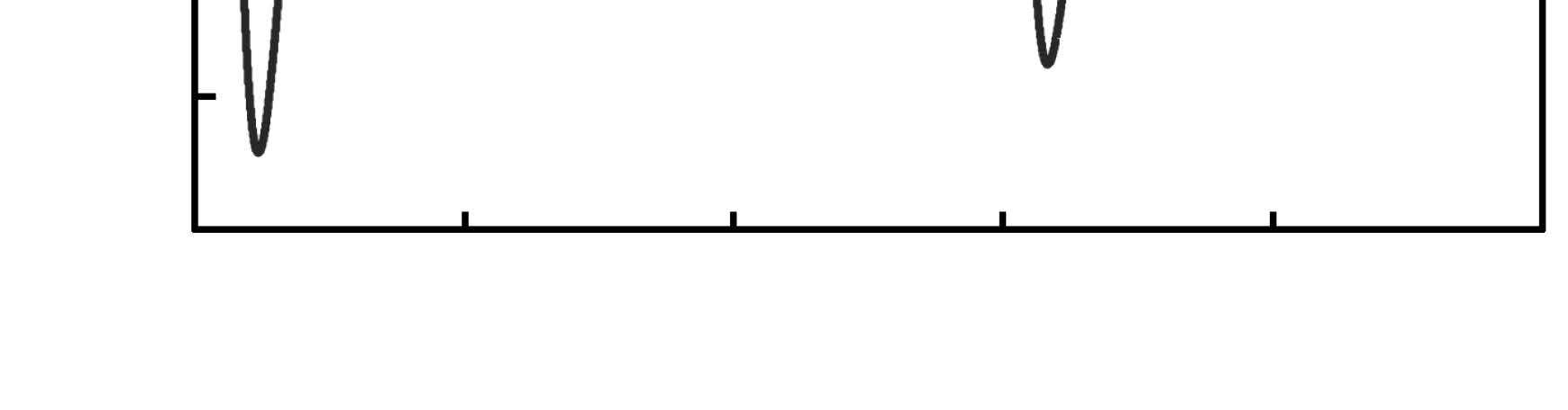
Case 1. Without solving the IID $\eta_{d}$,we directly set $\eta_{d}=0$,and simultaneously select $R=1$,$\omega=0.5$. Under this circumstance,we mean to stabilize the internal dynamics to zero. However,from the simulation results (Fig.2 and 3),it can be seen that the tracking performance is poor,and the internal dynamics does not converge to zero at all. From this simulation case,we can see that it is unavoidable to solve the IID $\eta_{d}$ which plays an important pole in acquiring fine output tracking performance.

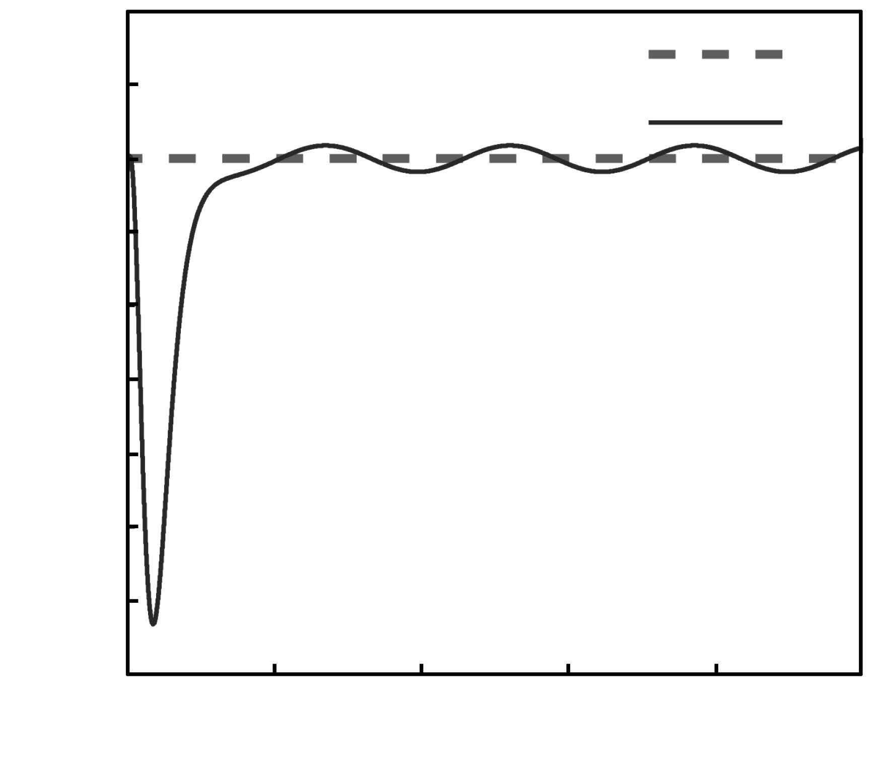
Case 2. The IID $\eta_{d}$ is solved via the SSC method,and the amplitude $R$ and the frequency $\omega$ of the desired output trajectory $y_{d}$ switch from $1$ to $1.2$ and $0.5$ to $1$, respectively,at random time $T=25+5\times {rand}(1)$. Such switches may occur in the case of obstacle avoidance. From the simulation results (Figs. 4-6),it can be concluded that the output tracking performance is fine,and the internal dynamics can track its corresponding casual IID despite the fact that the amplitude and frequency of the desired signal $y_{d}$ change at any random time.

Through the simulation cases,the following conclusions can be drawn:

1) It is necessary to solve the IID which is fundamental to achieve desired tracking performance when dealing with non-minimum phase systems.

2) Based on output redefinition,the proposed output-feedback DSC controller for nonlinear non-minimum phase systems is effective.

Ⅶ. Conclusion

The paper has proposed an output-feedback tracking control scheme for a class of nonlinear non-minimum phase systems via DSC method. After output redefinition,we directly design control law for the external dynamics rather than the internal dynamics,because the internal dynamics will get stable with the stability of the external dynamics. The proposed output-feedback DSC controller not only drives the system output signal to track the desired trajectory,but also makes the unstable internal dynamics to follow its corresponding bounded IID. The stability analysis has proved that the tracking errors can converge to zero and the closed-loop system is semi-globally stable. The effectiveness of the proposed output-feedback DSC control scheme has been illustrated by the simulation results.