 2016, Vol.3


HETEROGENEOUS wireless sensor network (HWSN) is a
wireless ad hoc network which is consisted of a large number of
different types of sensor nodes. Unlike homogeneous WSN,nodes are
randomly deployed in the monitored area,which are equipped with
extremely different energy. Heterogeneity can sharply increase the
average delivery rate and the network lifetime if nodes are
deployed as an effective network
Topology control is one of the most important techniques used for
reducing energy consumption and maintaining network
connectivity
In this paper,a clustering-tree topology control algorithm based on energy forecast (CTEF) is introduced for HWSN in order to solve the problem how to save energy and ensure the network load balancing. In HWSN,forecasting the energy consumption per round during the network lifetime and the actual lifespan of network is much more difficult than homogeneous WSN. We propose CTEF algorithm for solving this problem in an efficient way in terms of the estimated difference between the ideal average residual energy and the actual average residual energy to obtain the average energy of network at the next round. The cluster heads are selected depending on the synthesized cost function and their distance,while the clusters are formed by combining with the factors of the energy,distance and link quality.Moreover, the burden of the cluster-head,several non-cluster head nodes in each cluster are chosen as the relay nodes for transmitting data through multi-hop communication. The performance of CTEF is evaluated and found better than other typical protocols and algorithms via simulation.
The rest of this paper is organized as follows. In Section II,we present related work on clustering algorithms for HWSN. Section III describes the heterogeneous model for wireless sensor network. Furthermore,a clustering tree topology algorithm based on energy forecast is proposed in detail and our simulation results show the performance of the proposed algorithm in Sections IV and V, respectively. Finally,we conclude our paper in Section VI.
II. RELATED WORKClustering scheme is one of the most typical ways for topology
control in WSN. Most of cluster-based algorithms always adopt data
fusion scheme and pursue clustering objectives
Recently,quite a lot of energy-oriented algorithms for HWSN are
proposed. For instance,energy efficient heterogeneous clustered
(EEHC) algorithm is proposed based on the three-level network model
in
An efficient and dynamic clustering scheme (EDCS) is proposed for
multi-level heterogeneous wireless sensor networks in
The main difference between what we mentioned in above and our solution described in the following lies in network model. We use more general network model with multi-level heterogeneous features,which means we need to further take into account more complicated and actual factors and situations. As a clustering-tree topology control scheme,CTEF has advantages both from the clustering and tree algorithms. Energy consumption can be predicted more accurately in each round during the network lifetime,which results to be more reasonable for cluster-head selection and cluster formation. In addition,to avoid excessive energy consumption from the cluster-head,several non-cluster head nodes are chosen to be the relay node to further reduce the burden of each cluster-head. That is why CTEF with multi-hop communication can have longer lifetime.
III.HETEROGENEOUS MODEL FOR WSN A.Types of Heterogeneity and Impact on WSNUnlike homogeneous WSN,there are many special features in HWSN.
Generally,the common types of heterogeneity in WSN are classified
as follows
1) Computational heterogeneity: Different nodes have different capabilities to store information or deal with emergent events. Some super or advanced nodes have more powerful processor and memory than any other normal nodes. With high performance hardware,these nodes which own powerful computational capabilities can provide more and more ability for data storage and complex data processing,e.g.,data fusion is executed when the node receives a large number of data at the same time.
2) Link heterogeneity: With similarity to the computational heterogeneity,due to the powerful electronic devices,some nodes have more channels,higher bandwidth and longer communication distance than normal nodes. So they can provide more reliable and robust data transmission network.
3) Energy heterogeneity: It is the most important and key point in these three common types of heterogeneity. Computational heterogeneity and link heterogeneity always lead to consuming more energy than nodes in homogenous network so that their lifetime will fall down quickly. Energy heterogeneity can be represented as which nodes are equipped with different times of energy virtually.
In homogeneous WSN,each node has the same computational and communication capability,initial energy,and dissipates equivalent energy per round. However,the practical WSN is always composed of multiple sensors which are given different processing capabilities and initial energy. Each node has multi-level power options such that it consumes different energy per round in the normal working time depending on its current power level. Also, the link quality and packet loss rate should be taken into account for HWSN firstly because it could easily exist in such a complicated wireless situation. In addition,the interference can happen among nodes and clusters. Thus,the heterogeneous WSN with limitations is more suitable for research and more approximated to actual network.
B.Network ModelAssume that$N$ sensor nodes,which are all different from each other,are dispersed uniformly in an$M \times M$ square region. Besides,it has some features as follows:
1) Each node is equipped with a different initial energy over the interval of$[E_0,E_0(1+\lambda)]$,where $E_0$ is the lower bound and parameter$\lambda$ is a constant$(\lambda>0)$,which determines the value of the maximal initial energy;
2) The communication cost is different between nodes,and link quality and packet loss rate are arbitrary values in the interval of$(0,1]$;
3) The non-cluster heads cannot be allowed to communicate with the base station (BS) directly,only the cluster-head can send data directly to the base station;
4) The fusion strategies are executed by the cluster-head to aggregate correlated data before transmitting to the base station;
5) The distance between nodes is calculated by the received signal strength indicator (RSSI);
6) The interference can be neglected by using CSMA/CA in MAC layer.
7) The sink node is located at the center of region,and it is not restricted by energy,etc.
C.Energy ModelIn this paper,we use the same radio energy dissipation model that
was proposed in
| $ {E_{CH}} = l{E_{\rm elec}}\left(\frac{N}{k} - 1\right) + l{E_{DA}}\frac{N}{k} + l{E_{\rm elec}} + l{\xi _{\rm mp}}d_{{\rm to}BS}^4, $ | (1) |
| $ {E_{{\rm non}CH}} = l{E_{\rm elec}} + l{\xi _{fs}}d_{{\rm to}CH}^2, $ | (2) |
where$E_{CH}$ and$E_{{\rm non}CH}$ denote the energy dissipated within the cluster-head and non-cluster head during a round when sending$l$ bits message respectively,$E_{\rm elec}$ is the energy dissipated per bit to run the transmitter or the receiver,$E_{DA}$ is the data aggregation cost spent in the clusters,$\xi_{fs}$ and $\xi_{\rm mp}$ is the transmitting and amplifying parameter,$k$ is the number of clusters,$N$ is the number of sensor nodes,$N/k$ denotes the average number of nodes in a cluster,$d_{{\rm to}BS}$ is the average distance between the cluster-head and the base station,and$d_{{\rm to}CH}$ is the average distance between a cluster member and its cluster-head.
If the$N$ nodes are uniformly distributed in the$M \times M$
square area,$d_{{\rm to}BS}$ and$d_{{\rm to}CH}$ can be shown
respectively
| $ {{\rm d}_{{\rm to}BS}} = \int_{{M^2}} {\sqrt {{x^2} + {y^2}} } \frac{1}{{{M^2}}}{\rm d}{M^2} = 0.3825M, $ | (3) |
| $ {{\rm d}_{{\rm to}CH}} = \sqrt {\iint {({x^2} + {y^2})\rho (x,y){\rm d}x{\rm d}y} } = \frac{M}{{\sqrt {2\pi k} }}. $ | (4) |
Our proposed algorithm CTEF aims to find an effective way for HWSN
to save energy consumption and prolong the network lifetime. We
can clearly see from

|
Download:
|
| Fig. 1 The flow chart of CTEF algorithm. | |
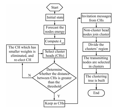
Due to the limitations from node itself,how to effectively use energy is one of the most important issues in the heterogeneous wireless networks. Generally,the average energy estimation is conducive to reduce the transmission of messages and decrease the energy consumption. In this paper,the average residual energy of network is estimated through the ideal average residual energy, which needs the so-called ideal lifetime.
Theorem 1. In the practical applications (the death of nodes is not at the same time,which is different from the ideal scenarios),the network lifetime is longer than the so-called ideal lifetime,i.e.,$R = \frac{{\Delta {E_{T1}}}}{{{E_{\rm round1}}}} + \frac{{\Delta {E_{T2}}}}{{{E_{\rm round2}}}} +\cdots + \frac{{\Delta {E_{Tm}}}}{{{E_{{\rm round}m}}}} > \frac{{{E_{\rm total}}}}{{{E_{\rm round}}}}$ $ (m = 1,2,...)$,where$m$ is a variable and denotes that the lifetime is divided into$m$ phases by changing the number of sensor nodes.${E_{{\rm round}m}}$ and $\Delta {E_{Tm}}$ are the energy consumption of the network in each round and the network total energy consumption at the$m$-th stage,respectively,$E_{\rm round}$ is the ideal energy consumption per round and$E_{\rm total}$ is the total initial energy.
Proof. The network is composed of$N$ sensor nodes,each node is equipped with a different initial energy over the interval of $[E_0,E_0(1+\lambda)]$. Thus,the total initial energy of the heterogeneous network is given by:
| $ \label{eqn_5} {E_{\rm total}} = \sum\limits_{i = 1}^N {{E_0}(1 + {\lambda _i})} = {E_0}\left(N + \sum\limits_{i = 1}^N {{\lambda _i}} \right). $ | (5) |
Meanwhile,energy dissipated in every cluster during a round can
be obtained by (1) and (2),and the total energy of the$k_{\rm
opt}$ clusters dissipated during a round
| $ {E_{\rm round}} ={k_{\rm opt}}{E_{\rm cluster}}\notag\\ = {k_{\rm opt}}\left[{E_{CH}} + \left(\frac{N} {{{k_{\rm opt}}}} - 1\right){E_{{\rm non}CH}}\right]\\ \approx \left[N(2{E_{\rm elec}} + {E_{DA}} + {\xi _{fs}}d_{{\rm to}CH}^2) + {k_{\rm opt}}{\xi _{\rm mp}}d_{{\rm to}BS}^4\right]. $ | (6) |
According to (6),we can easily know that the energy consumption of each round is proportional to the number of nodes.
Afterwards,the network lifetime $R_{\rm life}$ can be calculated as follows:
| $ {R_{\rm life}} = \frac{{{E_{\rm total}}}}{{{E_{\rm round}}}}. $ | (7) |
Equation (7) represents that$R_{\rm life}$ is inversely proportional to$E_{\rm round}$ with the same energy,which means the more the energy consumption in each round,the less the network lifetime. Without loss of generality,the network lifetime $R_{\rm life}$ is inversely proportional to the number of nodes.
If the initial total energy of the network$E_{\rm total}$ can be divided into$m$ parts uniformly,which can be denoted by $\Delta {E_T}$,we have
| $ {R_{\rm life}} = \frac{{{E_{\rm total}}}}{{{E_{\rm round}}}} = \frac{{\Delta {E_T}}}{{{E_{\rm round1}}}} + \frac{{\Delta {E_T}}}{{{E_{\rm round2}}}} + \cdots + \frac{{\Delta {E_T}}}{{{E_{{\rm round}m}}}}. $ |
In the ideal environment,the energy consumption in each round can be regarded as equal,and the so-called ideal lifetime is
| $ {R_{\rm ideallife}} = \ \frac{{\Delta {E_T}}}{{{E_{\rm idealround1}}}} + \frac{{\Delta {E_T}}}{{{E_{\rm idealround2}}}}\\ \ + \cdots{+}\frac{{\Delta {E_T}}}{{{E_{{\rm idealround}m}}}} = m\frac{{\Delta {E_T}}}{{{E_{\rm idealround1}}}}, $ |
where$E_{\rm ideallife}$ is the energy consumption of each round at the ideal situation. Furthermore,the actual lifetime is
| $ {R_{\rm actuallife}}=\ \frac{{\Delta {E_T}}}{{{E_{\rm actualround1}}}} + \frac{{\Delta {E_T}}}{{{E_{\rm actualround2}}}}\\ \ + \cdots{+} \frac{{\Delta {E_T}}}{{{E_{{\rm actualround}m}}}}, $ |
where$E_{\rm actuallife}$ is the energy consumption of each round at the actual situation. It states that with the death of nodes,the energy consumption of each round will be reduced, and the lifetime will be increased. Then,we have
| $ \frac{{\Delta {E_T}}}{{{E_{{\rm actualround}i}}}} > \frac{{\Delta {E_T}}}{{{E_{{\rm idealround}i}}}}. $ |
Therefore,with the decrease of the number of nodes,the lifetime
will increase in the practical applications,which is longer than
the so-called ideal network lifetime. The changes of lifetime can be
seen intuitively in

|
Download:
|
| Fig. 2 Curve comparison chart between the so-called ideal lifetime and the actual lifetime. | |
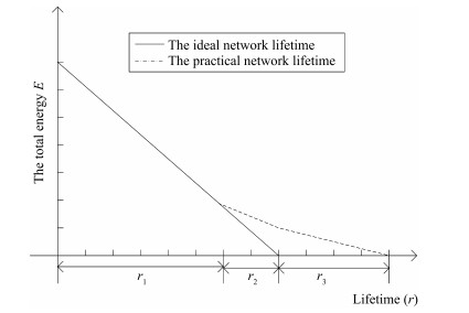
According to (5) and (7),we can obtain
| $ {\bar E_{\rm ideal}}(r) = \frac{1}{N}{E_{\rm total}}\left(1 - \frac{r}{{\alpha {R_{\rm life}}}}\right), $ | (8) |
where${\bar E_{\rm ideal}}(r)$ is the ideal average residual energy of the network in the$r$-th round,$R_{\rm life}$ is the total lifetime and$\alpha$ is a correction factor that satisfies $\alpha=1+0.1\lambda+0.001N$.
Definition 1.$e(r)$ is denoted as the difference between the ideal average energy of the network and the actual average energy of the network.
Lemma 1. Central limit theorem: suppose there are $n$
mutually independent random variables,and$n$ tends to infinity,
then its sub-sample mean is subject to the normal
distribution
Theorem 2. For wireless sensor networks,the mean of the samples from the average energy difference between the ideal and actual scenarios is subjected approximately to the normal distribution.
Proof. Assume that ${X_{{e_1}}},{X_{{e_2}}},...,{X_{{e_k}}}$ denotes the energy difference sequence,and$E({X_{{e_i}}}) = \mu $,$D({X_{{e_i}}}) = {\sigma ^2}$. According to lemma 1,there exists an arbitrary value of$x_e$:
| $ \mathop {\lim}\limits_{k \to \infty } p\left\{ {\frac{{\sum\limits_{i = 1}^k {{X_{{e_i}}}} - k\mu }}{{\sqrt k \sigma }} \le {x_e}} \right\} = \frac{1}{{\sqrt {2\pi } }}\int_{ - \infty }^{{x_e}} {{{\rm e}^{ - \frac{{{t^2}}}{2}}}{\rm d}t}. $ | (9) |
From (9),when the value of$k$ is large,which $k$ is the number of the samples of energy difference,$\sum\nolimits_{i = 1}^k {{X_{{e_r}}}} $ follows the normal distribution${\rm N}(k\mu ,k{\sigma ^2})$,then by transforming we can get
| $ \mathop {\lim}\limits_{c \to \infty } p\left\{ {\frac{(\frac{{\sum\limits_{i = 1}^c {{X_{{e_r}}}} }}{c} - \mu )}{(\frac{\sigma }{{\sqrt c }}) \le {x_e}}} \right\} = \frac{1}{{\sqrt {2\pi } }}\int_{ - \infty }^{{x_e}} {{{\rm e}^{ - \frac{{{t^2}}}{2}}}{\rm d}t}, $ | (10) |
where$c$ is the number of sample nodes.
Equation (10) shows that the mean of the samples from the energy difference$\frac{1}{c}\sum\nolimits_{i = 1}^c {{X_{{e_r}}}}$ is subjected approximately to the normal distribution${\rm N}(\mu,\frac{{{\sigma ^2}}}{c})$,which means that the mean of energy difference sequence is similar to the normal distribution.
The average residual energy of the network${\bar E_{\rm ideal}}(r)$ is an ideal estimation value which is not suitable in practice. So in this paper,the difference between the ideal and the actual average residual energy of the network is used to predict the energy at the$r$-th round,which is given by
| $ {\bar E_{\rm total}}(r) = {\bar E_{\rm ideal}}(r) + e(r), $ | (11) |
where$e(r)$ is the difference between the ideal and the actual average residual energy of the network,as defined in Definition 1. The mean of the sub-sample$u'$ is subjected approximately to the normal distribution,which means${\mu '}\sim {\rm N}({\bar \mu}', {\sigma ^2})$.
| $ {\bar \mu '} = \frac{{\mu _1' + \mu _2' + \cdots + \mu _k'}}{k}, $ | (12) |
| $ {\sigma ^2} = \frac{{{{({{\bar \mu }'} - \mu _1')}^2} + {{({{\bar \mu }'} - \mu _2')}^2} + \cdots + {{({{\bar \mu }'} - \mu _k')}^2}}}{k}, $ | (13) |
where${\bar \mu '}$ is the expectation and$\sigma ^2$ is the variance.
At the first and the second round,both differences$e(1)$ and $e(2)$ can be obtained directly. But they cannot compose the normal distribution because of few numbers. So firstly,suppose that the energy difference$e(r)$ follows the normal distribution. Then we can get a confidence interval to select eight numbers randomly and compose a sample with$e(1)$ and$e(2)$. Secondly,three samples among$C_{10}^3$ cases existed are extracted to get the mean of the samples$u'$,respectively. Furthermore,we can obtain a normal distribution about the mean of the sample according to Theorem 2 and calculate the energy difference$e(r)$ at the next round through a confidence interval. Finally,when the round$r$ is larger than 10, samples can be extracted directly to get the mean sequence,and the energy difference $e(r)$ at the$r$-th round can be predicted to calculate the average residual energy of the network.
B.Cluster-head SelectionTo have network load balancing and prolong the lifetime as far as possible,we combine three factors (i.e.,node energy,link quality and packet loss rate) which are called the cost to evaluate the node performance comprehensively. The selection mechanism is based on the complexity of the actual network. The best nodes are selected as the cluster-head by cost function. The cost function is given by
| $ C=\frac{1}{\beta (\frac{{E_{\rm res}}}{{{\bar E}_{\rm total}(r)}}) + ({p_{\rm link}} + (\frac{1}{{p_{\rm loss}}})) \cdot \frac{(1 - \beta )}{2}}, $ | (14) |
where$\beta$ is the weighted coefficient and $\beta \in (0,1)$, $E_{\rm res}$ is the residual energy of the node,$p_{\rm link}$ is the link quality,$p_{\rm loss}$ is the packet loss rate,${p_{\rm link}},{p_{\rm loss}} \in (0,1]$. And$p_{\rm link}$ is inversely proportional to$p_{\rm loss}$,which means if the link quality is higher,the packet loss rate is lower. Equation (14) shows that the node which has more energy,higher link quality and lower packet loss rate,will be more likely to be selected as the cluster-head. Compared to other nodes,these cluster heads will have more available energy,while their rate of transmitting data will be higher. Meanwhile,the remaining nodes collect data in their monitoring region as the member of each cluster. So the network performance will be better.
In this paper,the method of $N$-order nearest neighbor in
After the node has been selected as the cluster-head,it needs to broadcast message to other nodes in the network and waits for response. Generally,the cluster-head can be seen at the center of the cluster region because the communication range of nodes is always a circle. Once each non-cluster head node receives invitation messages from multiple cluster heads,it computes the distance$d(i,j)$ between the sender and the receiver based on the receiver signal strength indicator (RSSI). In order to help cluster formation,a method is introduced to guide the non-cluster head nodes to choose the most suitable cluster-head,which depends on the energy in cluster-head,the link quality between the cluster-head and the non-cluster head nodes,and the distance $d(i,j)$. Then we have
| $ F(i,j,r) = \frac{{E_{\rm res}^j{p_{\rm link}}}}{{d(i,j)}}, $ | (15) |
where$F(i,j,r)$ is the value between the cluster-head$j$ and the non-cluster head nodes$i$ in the$r$-th round,$E_{\rm res}^j$ is the residual energy of the cluster-head$j$ in the$r$-th round, $p_{\rm link}$ is the link quality between nodes,and$d(i,j)$ is the distance between$i$ and$j$.
Equation (15) shows that if a cluster-head owns more residual energy $E_{\rm res}^j$ and higher link quality between the cluster-head and the non-cluster head nodes,it will be more likely to attract a non-cluster head node to join. Likewise,the distance$d(i,j)$ can also be used to determine which cluster to join for the non-cluster head node. It means that the longer distance between the cluster-head and the non-cluster head nodes,the less possibility the non-cluster head nodes to join.
D.Tree Formation within ClusterClustering algorithm is still in line with the purpose of load balancing. However,if a cluster has too many members,the cluster-head will consume too much energy to bear more loads to communicate with the cluster members. So a way to search transferring nodes (these nodes will be executing data fusion) from cluster members is proposed which can construct a tree in the cluster. It aims to reduce the energy consumption and prolong the lifetime because of sharing the load of cluster heads. The mathematical expression can be denoted by
| $ z=\min(\Delta E) =\min\sigma _{\Delta E}^2\notag\\ = \min\left(\frac{1}{x}\sum\limits_{i = 1}^x {{{\left(E_{\rm res}^i - {{\bar E}_{\rm total}}(r)\right)}^2}} \right), $ | (16) |
where$z$ is an objective function,$x$ is the number of cluster members. The final purpose served by (16) is to balance the energy consumption in clusters and all the nodes can be dead at the same time possibly. It means that the residual energy$E_{\rm res}^i$ needs to be equal to the network average energy${\bar E_{\rm total}}(r)$ as much as possible in the$r$-th round.
On the other hand,after the cluster formation,a cluster-head can
be seen as the circle center and$L_2$ is the radius to divide the
cluster area into two parts,i.e.,a circle and an approximate ring.
It is shown in

|
Download:
|
| Fig. 3 Division of area about tree formation within cluster. | |
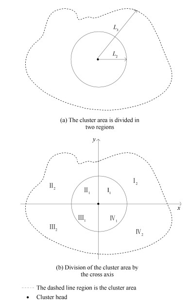
| $ \omega = \frac{\gamma }{{{E_{\rm res}}}} + \frac{{1 - \gamma }}{v}\sum\limits_{i = 1}^v {{{({d_i} - {d_{iCH}})}^2}}, $ | (17) |
where$\gamma$ is a weighted variable,$v$ is the number of nodes in each region,$d_i$ is the distance between nodes,$d_{iCH}$ is the distance between nodes and the cluster-head. $\frac{1}{v}\sum\nolimits_{i = 1}^v ({d_i}$$-$${d_{iCH}})^2$ is a variance of the distance,which means that the lower variance of node$i$,the more uniform distribution around the node$i$. From (17),we can see that if a node has more energy and less distance variance to the cluster-head,it will be more likely to become a relay node.
Algorithm 1. Pseudo-code of the CTEF algorithm
Require: A HWSN is represented by graph$G(V,E)$,$N$ is the number of nodes,$A$ is the rectangle region of the HWSN,and $e[r]$ is the residual energy of the network at$r$-th round.
1.$G(V,E)$ is initialized with $N$ and $A$;
2.$k_{\rm opt}$ is calculated by using $N$-order nearest neighbor;
3. while there exists an alive node
4.$//$ Generate cluster heads
5. if $r \le 2$ then
6. Calculate$e[r]$;
7. else if $r \ge 3$ and $r \le 10$
8. Generate randomly$e$ with length$(10 - r)$;
9. Calculate mean with any three samples;
10. Calculate $e[r]$ using Theorem 2;
11. else
12. Calculate $e[r]$ with its normal distribution;
13. end if
14. for $i=1$ to$n$ do
15. Calculate value of node$(i)$ with (14);
16. end for
17. Sort the nodes' values in descending order;
18. Switch the first$k_{\rm opt}$ node$(s)$ to cluster-head;
19.$//$ Generate cluster
20. while $((u,v) \in E)$ and ($i$ is not a cluster-head, $j$ is a cluster-head)
21. Calculate F(i,j,r) with equation (15);
22. if F(i,j,r) is shortest for any$v$} then
23.$i$ becomes a member of cluster with$j$;
24. end if
25. end while
26.$//$ Generate tree in each cluster
27. for all $u$ in the set of clusters
28. Divide cluster$u$ into 8 parts;
29. Node$v$ in each part becomes the relay node in terms of the shortest value$\omega$;
30. Connect the relay nodes with the shortest paths;
31. Connect the other nodes to$v$ in each part;
32. end for
33. if node$i$ is dead
34. Calculate$k_{\rm opt}$;
35. end if
36. end while
E.The Panorama of Proposed Algorithm and Its AnalysisAs described in above,we have to design such a series of complex processes to resolve energy consumption problem for HWSN to prolong the network lifetime. The pseudo-code is given in Algorithm CTEF to show the panorama of the proposed algorithm. In addition,we prove the time complexity of the CTEF is${\rm O}(n^2)$ through Theorem 3.
Theorem 3. The time complexity of the CTEF algorithm is${\rm O}(n^2)$.
Proof. As discussed above,the CTEF mainly contains 4 phases: the average energy estimation,the cluster-head selection, the cluster formation and the tree formation within the cluster. See pseudo-code of the CTEF,we only care about the process with loop. In cluster-head selection,the time complexity is determined by merge sort,which has the worst time complexity${\rm O}(n\log n)$. On the other hand,in cluster formation and tree formation within cluster phase,the time complexity is subjected to the computational complexity of$F(i,j,r)$ and$\omega$ respectively,and both them have the worst time complexity of order${\rm O}(n^2)$. The rest of the process has time complexity at most${\rm O}(n)$. Therefore,the final time complexity of the CTEF algorithm is${\rm O}(n^2)$.
V.SIMULATION RESULTS A.Parameters SetupIn this section,the performance of CTEF algorithm is evaluated in
the heterogeneous wireless sensor networks. As shown in
|
|
Table I Results Summary |
Due to the energy limitation,the lifetime is the one of the most important performance criteria to verify whether the proposed algorithm is useful. So,we take into account the influence of network lifetime within different number of nodes and energy parameter$\lambda$ (set multi-level energy via$\lambda$) using the CTEF to compare with LEACH,EDFCM and EDCS. Moreover,similar with performance of energy,throughput,i.e.,number of data packets received at the base station is also considered to evaluate our proposed algorithm. On the other hand,there are some sensitive parameters in CTEF which should be analyzed carefully because it may influence the simulation results. The heterogeneity and practical scenarios make the experiments more complicated. Therefore,we not only discuss the impact of the distance parameters$L_1$ and$L_2$ respectively,but also care about the influence of link quality and packet loss rate. In addition, analyzing the parameters of Algorithm 1,we even discuss the performance of our proposed algorithm within different lifetime (i.e.,time for first node to die and time for all nodes to die).
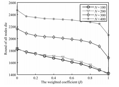
B.Analysis of Sensitivity ParametersIn order to keep simulation results objective and effective,i.e.,
random uncertain factors,the average result is evaluated by
multiple experiments with$\lambda=2.0$. Figs. 4 and 5 show the
influence about the link quality and packet loss rate by changing
the weighted coefficient$\beta$.

|
Download:
|
| Fig. 4 The time for all nodes to die under different weighted coefficient | |

|
Download:
|
| Fig. 5 The time for the first node to die under different weighted coefficient. | |
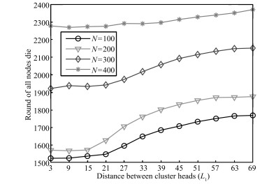
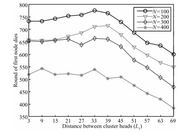
Figs. 6 and 7 illustrate the impact of distance$L_1$ among cluster
heads on the network lifetime with different nodes. From

|
Download:
|
| Fig. 6 The time for all nodes to die under different L1. | |
In

|
Download:
|
| Fig. 7 The time for the first node to die under different L1. | |
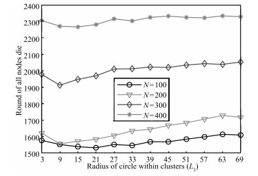
Figs. 8 and 9 denote the impact of the circle radius$L_2$ on the
network lifetime with different nodes.

|
Download:
|
| Fig. 8 The time for all nodes to die under different L2. | |

|
Download:
|
| Fig. 9 The time for the first node to die under different L2. | |
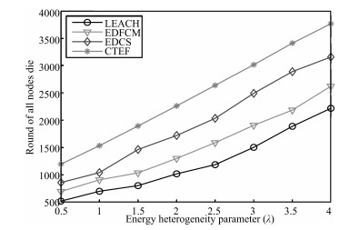
In this paper,the performance of the CTEF algorithm is verified
through comparing with LEACH,EDFCM and EDCS algorithms in the
network lifetime and the number of data packets received at the base
station.

|
Download:
|
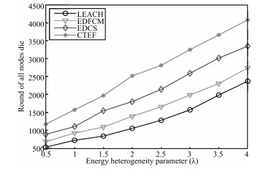
| Fig. 10 All nodes die with different λ (N = 100). | |

|
Download:
|
| Fig. 11 All nodes die with different λ (N = 200). | |

|
Download:
|
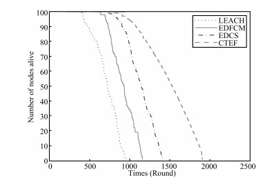
| Fig. 12 The network lifetime (N = 100). | |
As we said before,we have known that our CTEF has longer lifetime
to meet the purpose of saving energy and prolonging the network
lifespan. Furthermore,because the cluster-head selection and
cluster formation is associated with the link quality and packet
loss rate,we want to see whether the link quality and packet loss
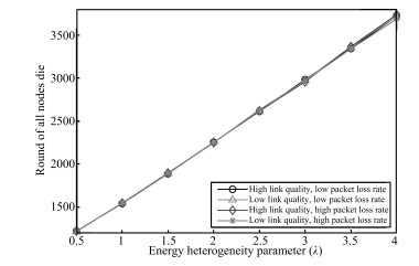
rate can affect the network lifetime. From

|
Download:
|
| Fig. 13 The impact of link quality and packet loss rate on lifetime with different λ. | |
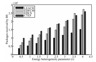
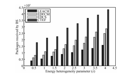
Finally,we pay attention to data packets which are received at base
station (BS) under all kinds of these protocols.

|
Download:
|
| Fig. 14 Packets received in BS (N = 100). | |

|
Download:
|
| Fig. 15 Packets received in BS (N = 200). | |
In this paper,CTEF,a clustering-tree topology control algorithm based on the energy forecast is proposed for heterogeneous wireless sensor networks. It solves the problem of energy consumption through considering the energy and link heterogeneity. The network average energy at the next round is estimated by the difference between the ideal and the actual average energy,while the energy difference is computed by the central limit theorem and the normal distribution. The cluster-head is selected by the cost which is expressed by the residual energy,link quality and packet loss rate. Moreover,the selected cluster heads are adjusted by considering the distance between cluster heads,and we also consider the residual energy and link reliability,etc.,to guide the cluster formation. Finally, CTEF searches the relay nodes within the cluster to transmit data to reduce the burden of the cluster-head. Simulation results show that CTEF is efficient for heterogeneous wireless sensor networks,and its performance about lifetime and throughput is better than LEACH, EDFCM and EDCS protocols.
| [1] | Bagci H, Korpeoglu I, Yazici A. A distributed fault-tolerant topology control algorithm for heterogeneous wireless sensor networks. IEEE Transactions on Parallel and Distributed Systems, 2015, 26(4):914-923 |
| [2] | Liu Y, Yang C L, Tang W K S, Li C G. Optimal topological design for distributed estimation over sensor networks. Information Sciences, 2014, 254(1):83-97 |
| [3] | Anastasi G, Conti M, Di Francesco M, Passarella A. Energy conservation in wireless sensor networks:a survey. Ad Hoc Networks, 2009, 7(3):537-568 |
| [4] | Lattanzi E, Regini E, Acquaviva A, Bogliolo A. Energetic sustainability of routing algorithms for energy-harvesting wireless sensor networks. Computer Communications, 2007, 30(14-15):2976-2986 |
| [5] | Fan T G, Teng G F, Huo L M. Deployment strategy of WSN based on minimizing cost per unit area. Computer Communications, 2014, 38:26-35 |
| [6] | Abbasi A A, Younis M. A survey on clustering algorithms for wireless sensor networks. Computer Communications, 2007, 30(14-15):2826-2841 |
| [7] | Kumar D, Aseri T C, Patel R B. EEHC:energy efficient heterogeneous clustered scheme for wireless sensor networks. Computer Communications, 2009, 32(4):662-667 |
| [8] | Heinzelman W B, Chandrakasan A P, Balakriahnan H. An applicationspecific protocol architecture for wireless microsensor networks. IEEE Transactions on Wireless Communications, 2002, 1(4):660-670 |
| [9] | Smaragdakis G, Matta I, Bestavros A. SEP:a stable election protocol for clustered heterogeneous wireless sensor networks. In:Proceedings of the 2nd International Workshop on Sensor and Actor Network Protocols and Applications. Boston, Massachusetts, USA, 2004. 223-233 |
| [10] | Qing L, Zhu Q X, Wang M W. Design of a distributed energy-efficient clustering algorithm for heterogeneous wireless sensor networks. Computer Communications, 2006, 29(12):2230-2237 |
| [11] | Hong Z, Yu L, Zhang G J. Efficient and dynamic clustering scheme for heterogeneous multi-level wireless sensor networks. Acta Automatica Sinica, 2013, 39(4):454-460 |
| [12] | Zhou H B, Wu Y M, Hu Y Q, Xie G Z. A novel stable selection and reliable transmission protocol for clustered heterogeneous wireless sensor networks. Computer Communication, 2010, 33(15):1843-1849 |
| [13] | Kuila P, Gupta S K, Jana P K. A novel evolutionary approach for load balanced clustering problem for wireless sensor networks. Swarm and Evolutionary Computation, 2013, 12(10):48-56 |
| [14] | Dabirmoghaddam A, Ghaderi M, Williamson C. On the optimal randomized clustering in distributed sensor networks. Computer Networks, 2014, 59(2):17-32 |
| [15] | Rajasegarar S, Leckie C, Palaniswami M. Hyperspherical cluster based distributed anomaly detection in wireless sensor networks. Journal of Parallel and Distributed Computing, 2014, 74(1):1833-1847 |
| [16] | Bandyopadhyay S, Coyle E J. Minimizing communication costs in hierarchically-clustered networks of wireless sensors. Computer Networks, 2004, 44(1):1-16 |
| [17] | Wang R X. Mathematical Statistics. Xi'an:Xi'an Jiaotong University Press, 1986. 245 |
| [18] | Hong Zhen, Yu Li, Zhang Gui-Jun. An adaptive distributed clustering routing protocol for wireless sensor networks. Acta Automatica Sinica, 2011, 37(10):1197-1205(in Chinese) |