Ⅰ. Introduction

In our daily lives,it is seen that a given task could be accomplished successfully if one could repeat the process for several times. In this case,one could learn important information from the past experiences and make an improvement in his/her current behavior. This intuitive cognition motivates the idea of iterative learning control (ILC),which was first proposed in ^[1] for robotics. Learning is the inherent characteristic of ILC different from other control strategies. That is,in ILC,the input and output information of past iterations,as well as the tracking objective,are used to formulate the input signal for the current iteration,so that the tracking performance could be improved iteration by iteration. Therefore,ILC is quite suitable for the systems that could complete some task over a finite time interval and repeat it again and again^[2,3,4]. It should be pointed out that stochastic ILC,which aims to the systems with stochastic noises,random disturbances and other uncertain factors,has attracted much attention from both scholars and engineers^[4].

To have more flexibility and tolerance,more and more systems are built following the networked control system scheme,where the plant and the controller are usually located at different sites and communicate with each other through wired/wireless networks. Due to the limitation of transmission bandwidth,the data burden is an important topic,while quantization of the actual signal before transmitting is a fair choice for many practical applications. Some previous studies are given in ^[5,6,7,8,9] covering estimation,identification,and control topics. However,limited literature is found from the perspective of quantized ILC.

Bu and co-workers made the first attempt on quantized ILC problem in ^[10],where the output measurements are quantized by a logarithmic quantizer and fed to the update law. By using sector bound method and conventional contract mapping method,it was shown that the tracking error converged to a bound depending on quantization density. However,it is noticed that the tracking error also depends on the output value. In other words,the larger the output measurement is,the larger the final tracking error bound is. In order to make a zero-error convergence of ILC based on quantized information,a possible way is proposed as follows. We first transmit the reference to the system before running the system for certain task. Then the system would make a comparison between its output and the given reference and quantize the error locally. It is the quantized error that is transmitted back to the controller later during the successive learning process. Based on this implementation,the tracking error converges to zero as iteration number goes to infinity. This is the mechanism used in the paper.

Here,the stochastic systems are taken into account. In this case,both stochastic noises from systems and quantization error are mixed and thus it is interesting whether a good performance could be achieved by ILC based on quantized information. To be specific,in this paper,we consider both linear and nonlinear stochastic systems and provide ILC update laws based on quantized error. In order to deal with the stochastic noises,a decreasing learning gain sequence is introduced to the update laws. As a result,it is proved that the input sequence would converge to the desired optimal input almost surely. That is,by minor modifications,ILC could behave well under both stochastic noises and quantization errors.

The rest of the paper is arranged as follows: Section Ⅱ gives the problem formulation and ILC law for stochastic linear systems; Section Ⅲ gives the detailed analysis of the convergence; Extension to nonlinear case is provided in Section Ⅳ; Ⅰ llustrative simulations are shown in Section Ⅴ; and Section ⅥI concludes the paper.

Ⅱ. Problem Formulation

Consider the following linear discrete-time stochastic systems:

$\begin{gathered} {x_k}(t + 1) = A(t){x_k}(t) + B(t){u_k}(t) + {w_k}(t + 1),\hfill \\ {y_k}(t) = C(t){x_k}(t) + {v_k}(t),\hfill \\ \end{gathered}$

(1)

where $k=1,2,...$ denotes iteration number,while $t=0,1,...,N$ denotes different time instances of one iteration. Here $N$ is the iteration length. ${x_k}(t) \in {R^n}$, ${u_k}(t) \in R$,and ${y_k}(t) \in R$ are state,input,and output,respectively. $A$,$B$,and $C$ are suitable matrices with appropriate dimensions. $w_k(t)$ and $v_k(t)$ are system noise and measurement noise,respectively.

The reference is denoted by $y_d(t)$,$t=\{0,1,...,N\}$. Then the tracking error is given by $e_k(t)=y_d(t)-y_k(t)$.

Let ${F_k}: = \sigma \{ {y_j}(t),{x_j}(t),{w_j}(t),{v_j}(t),0 \leqslant j \leqslant k,t \in \{ 0,...,N\} \} $ be the $\sigma$-algebra generated by $y_j(t)$,$x_j(t)$,$w_j(t)$,$v_j(t)$,$0\leq t\leq N$,$0\leq j\leq k$. Then the set of admissible controls is defined as $U = \{ {u_{k + 1}}(t) \in {F_k},\mathop {\sup }\limits_k {u_k}(t) < \infty ,{\text{a}}{\text{.s}}{\text{.}},t \in \{ 0,...,N - 1\} ,k = 0,1,2,...\} .$ From the definition of the set $U$,it is noticed that there are two requirements on the admissible control sequence $\{u_k(t), k=0,1,2,...\}$. One is that the input sequence should be bounded in the almost sure sense. The other one is that $u_{k+1}(t)$ should be ${F_k}$-measurable,i.e.,the input $u_{k+1}(t)$ could be expressed by the information in ${F_k}$ which is a basic requirement of ILC. Thus the set $U$ is compact.

The control objective is to find an input sequence $\{u_k(t),k=0,1,2,...\}\subset U$ to minimize the following averaged tracking errors,$\forall t\in\{0,1,...,N\}$

$V(t) = \mathop {\lim \sup }\limits_{n \to \infty } \frac{1}{n}\sum\limits_{k = 1}^n {{y_d}(} t) - {y_k}(t){^2}.$

(2)

For further analysis,the following assumptions are needed.

A1. The real number $C(t+1)B(t)$ coupling the input and output is an unknown nonzero constant,but its sign, characterizing the control direction,is assumed known. Without loss of any generality,it is assumed that $C(t+1)B(t)>0$ in the rest of the paper.

Remark 1. It is noted that $C(t+1)B(t)\neq 0$ is equivalent to claiming that the input/output relative degree is one. In the followings,without causing confusion,the symbol $C(t+1)B(t)$ will be abbreviated as $C^+B(t)$ for simplicity of writing.

Under A1 and the system (1),it is noted there exist suitable initial state value $x_d(0)$ and input $u_d(t)$ such that

$\begin{array}{*{20}{l}} {}&{{x_d}(t + 1) = A(t){x_d}(t) + B(t){u_d}(t),} \\ {}&{{y_d}(t) = C(t){x_d}(t).} \end{array}$

(3)

As a matter of fact,by A1,the following is a recursive solution to (3) with initial state $x_d(0)$, ${u_d}(t) = {({C^ + }B(t))^{ - 1}}({y_d}(t + 1) - C(t + 1)A(t){x_d}(t)).$

We formulate this fact into the following assumption.

A2. The reference $y_d(t)$ is realizable,i.e.,there is a unique input $u_d(t)$ such that

$\begin{gathered} {x_d}(t + 1) = A{x_d}(t) + B{u_d}(t),\hfill \\ {y_d}(t) = C{x_d}(t),\hfill \\ \end{gathered}$

(4)

with a suitable initial state $x_d(0)$.

A3. For each $t$ the independent and identically distributed (IID) sequence $\{w_k(t),k=0,1,...\}$ is independent of the IID sequence $\{v_k(t),k=0,1,...\}$ with ${\rm E}w_k(t)=0$,${\rm E}v_k(t)=0$,$\sup_k{\rm E}w_k^2(t)<\infty$,$\sup_k{\rm E}v_k^2(t)<\infty$, $\lim_{n\rightarrow\infty}\frac{1}{n}\sum_{k=1}^nw_k^2(t)=R_w^t$, and $\lim_{n\rightarrow\infty}\frac{1}{n}\sum_{k=1}^nv_k^2(t)=R_v^t$, almost surely (a.s.),where $R_w^t$ and $R_v^t$ are unknown.

Note that the noise assumption is made according to the iteration axis rather than the time axis,thus this requirement is not rigorous as the process would be performed repeatedly.

A4. The sequence of initial values $\{x_k(0)\}$ is IID with ${\rm E}x_k(0)=x_d(0)$,$\sup_k{\rm E}x_k^2(0)<\infty$,and $\lim_{n\rightarrow\infty}\frac{1}{n}\sum_{k=1}^nx_k^2(0)=R^0_x$. Further,the sequences $\{x_k(0),k=0,1,...\}$, $\{w_k(t),k=0,1,...\}$,and $\{v_k(t),k=0,1,...\}$ are mutually independent.

To facilitate the expression,denote $w_k(0)=x_k(0)-x_d(0)$. Then it is easy to define $\lim_{n\rightarrow\infty}\frac{1}{n}\sum_{k=1}^nw_k^2(0)=R_w^0$ to satisfy the formulation of A3. In other words,A4 can be compressed into A3.

Lemma 1. Consider the stochastic system (1) and tracking objective $y_d(t+1)$,and assume A1-A4 hold,then for any arbitrary time $t+1$,the index (2) will be minimized if the control sequence $\{u_k(t)\}$ is admissible and satisfies $u_k(i)\xrightarrow[k\rightarrow\infty]{}u_d(i)$, $i=0,1,...,t$. In this case,$\{u_k(t)\}$ is called the optimal control sequence.

The proof is given in Appendix A.

Ⅲ. ILC Design and its Convergence Results

In traditional ILC,the tracking error $e_k(t)$ is transmitted back for updating the input signal. In other words,the update law for input is

${u_{k + 1}}(t) = {u_k}(t) + {a_k}{e_k}(t + 1),$

(5)

where $a_k$ is learning step-size.

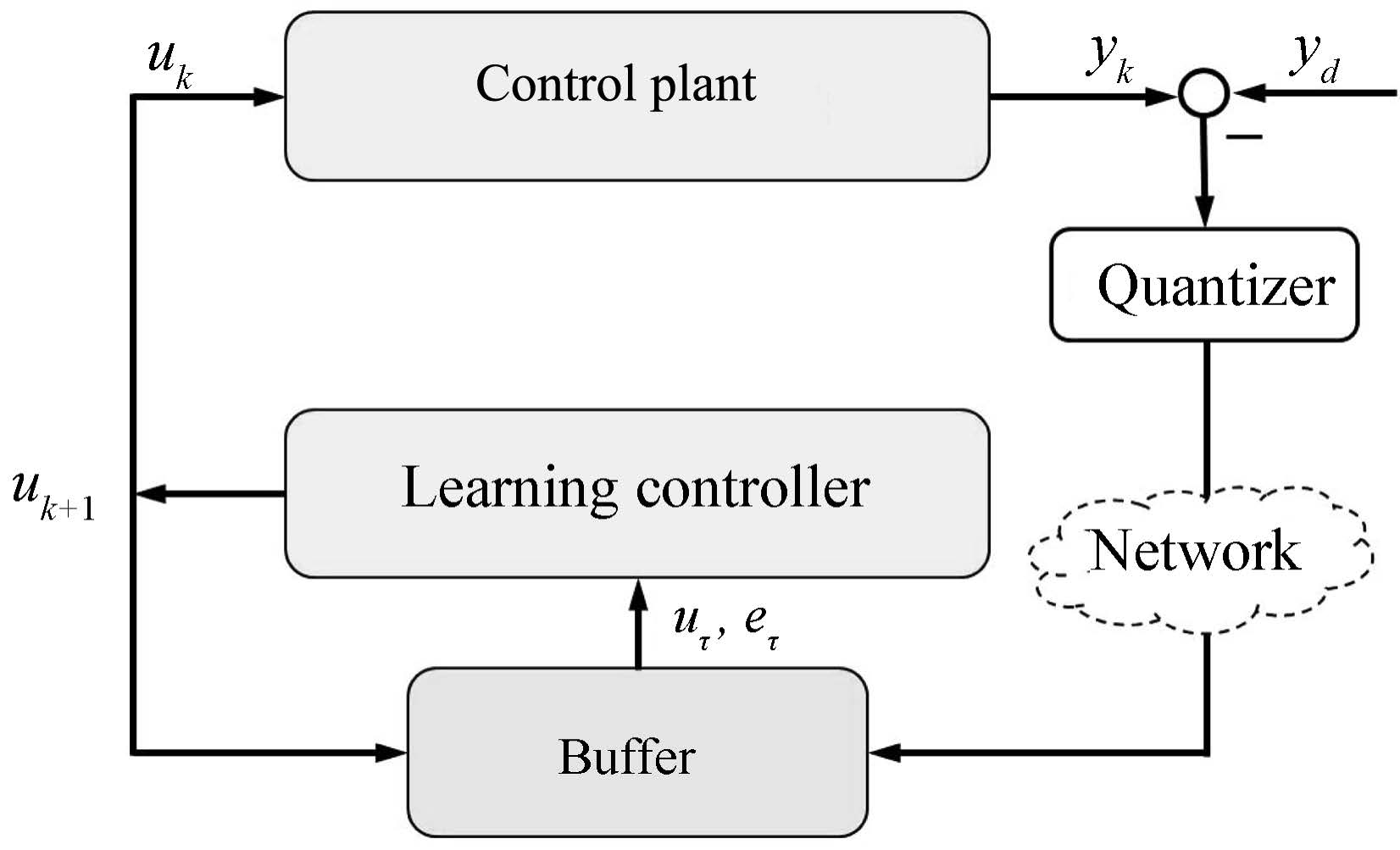
In this paper,we consider a networked implementation of the whole control system,i.e.,the plant and the controller are located in different sites as shown in Fig.1. To reduce transmission burden,for any specified tracking reference,we first transmit it to the plant before operating. Then the tracking error is generated,quantized,and transmitted back to the controller. Thus the delivery of the desired reference would need more efforts before starting learning. However,in the current implementation, the line from controller center to local plant site works well so that the input signal could be precisely transmitted. As one could see,the new desired reference could be delivered through this network.

The update law used in this paper is

${u_{k + 1}}(t) = {u_k}(t) + {a_k}Q({e_k}(t + 1)),$

(6)

where $a_k$ is learning step-size and ${Q}(\cdot)$ is a selected quantizer. In this paper,a logarithmic quantizer as in ^[11] is adopted,

$\begin{gathered} U = \{ \pm {z_i}:{z_i} = {\mu ^i}{z_0},i = 0,\pm 1,\pm 2,...\} \cup \{ 0\} ,\hfill \\ \quad 0 < \mu < 1,{z_0} > 0,\hfill \\ \end{gathered}$

(7)

where $\mu$ is associated with the quantization density. The associated quantizer ${Q}(\cdot)$ is given as

$Q(v) = \left\{ {\begin{array}{*{20}{l}} {{z_i},}&{if\frac{1}{{1 + \zeta }}{z_i} < v \leqslant \frac{1}{{1 - \zeta }}{z_i},} \\ {0,}&{ifv = 0,} \\ { - Q( - v),}&{ifv < 0,} \end{array}} \right.$

(8)

with $\zeta=(1-\mu)/(1+\mu)$. It is evident that the quantizer ${Q}(\cdot)$ in (8) is symmetric and time-invariant.

In ^[12],a sector bound method is proposed to deal with the quantization error. In this paper,specifically speaking,for a given quantization density $\mu$,we have

$\begin{align}\label{quanerror} {Q}(e_k(t))-e_k(t)=\eta_k^t\cdot e_k(t), \end{align}$

(9)

where $|\eta_k^t|\leq \zeta$ and $\zeta=(1-\mu)/(1+\mu)$.

Problem statements. Select suitable step-size $\{a_k\}$ and quantizer parameter $\mu$ such that the input sequence generated by update law (6) would minimize the tracking index (2) for stochastic linear system (1) under assumptions A1-A4.

The convergence of (6) is given in the following theorem.

Theorem 1. Consider stochastic linear system (1) and index (2),and assume A1-A4 hold,then the input generated by update law (6) with quantized tracking error is optimal according to Lemma 1 if the learning step-size $a_k$ satisfies $a_k>0$, $a_k\rightarrow0$,$\sum_{k=1}^{\infty}a_k=\infty$, $\sum_{k=1}^{\infty}a_k^2<\infty$ and the quantizer parameter $\mu$ is arbitrarily selected in the range $(0,1)$. In other words,$u_k(t)$ converges to $u_d(t)$ a.s. as $k\rightarrow\infty$ for any $t\in[0,N-1]$.

The proof is somewhat long and is given in Appendix B.

Remark 2. It is noted from Theorem 1 that the input sequence would converge to the optimal one no matter how dense the logarithmic quantizer is. In other words,the convergence is independent of $\zeta$ or $\mu$. This means that the algorithm can behave well even a rough quantizer is adopted,thus we may save much cost on devices. The inherent reason is that the quantization error is bounded by the actual tracking error. Consequently, larger tracking error means larger quantization error,however, this is acceptable because the learning is rough at this stage. While as the tracking error converges to zero,the quantization error also reduces to zero.

Remark 3. Because of the existence of stochastic noises,the actual tracking error would not converge to zero,which further leads to that the quantization error does not converge to zero. The sequence $\{a_k\}$ plays two roles here,one of which is to guarantee the zero-error convergence of the input almost surely, and the other one is to suppress the effect of stochastic noises and quantization errors as iteration number increases. However,it should be noted that the decreasing property of $a_k$ slows down the convergence speed of the proposed algorithm. This could be regarded as a trade-off of tracking performance and convergence speed.

Remark 4. Since the optimal tracking performance is achieved independent of quantizer,it leaves much freedom for the design of the algorithm. If the system is extended to MIMO case,where $C^+B(t)$ is a matrix,a learning gain matrix $L_t$ should be extra introduced as a learning direction satisfying that $L_tC^+B(t)$ is a square matrix and all its eigenvalues are positive. This condition is quite relaxed for stochastic systems.

Ⅳ Extension to Nonlinear Systems

In this section,we extend the linear time-varying system (1) to the following affine nonlinear systems with measurement noise

$\begin{array}{*{20}{l}} {}&{{x_k}(t + 1) = f(t,{x_k}(t)) + B(t,{x_k}(t)){u_k}(t),} \\ {}&{{y_k}(t) = C(t){x_k}(t) + {v_k}(t),} \end{array}$

(10)

where $f(t,x_k(t))$ and $B(t,x_k(t))$ are continuous functions. In addition,${x_k}(t) \in = {R^n}$,${u_k}(t) \in R$,and ${y_k}(t) \in R$. The control objective is to minimize the index (2).

The assumptions are modified as follows.

A5. The tracking reference $y_d(t)$ is realizable in the sense that there exist $u_d(t)$ and $x_d(0)$ such that

$\begin{array}{*{20}{l}} {}&{{x_d}(t + 1) = f(t,{x_d}(t)) + B(t,{x_d}(t)){u_d}(t),} \\ {}&{{y_d}(t) = C(t){x_d}(t).} \end{array}$

(11)

A6. The functions $f(\cdot,\cdot)$ and $B(\cdot,\cdot)$ are continuous with respect to the second argument.

A7. The real number $C(t+1)B(t,x_d(t))$ coupling the input and output is an unknown nonzero constant but its sign is assumed known prior. Without loss of generality,it is assumed $C^+B_d(t):= C(t+1)B(t,x_d(t))>0$. Here $x_d(t)$ is the solution of the system (11).

A8. The initial values can asymptotically be precisely reset in the sense that $x_k(0)\rightarrow x_d(0)$ as $k\rightarrow\infty$.

A9. For each $t$,the measurement noise $\{v_k(t)\}$ is a sequence of IID random variables with ${\rm E}v_k(t)=0$,$\sup_k{\rm E}v_k^2(t)<\infty$,and $\lim_{n\rightarrow\infty}\frac{1}{n}\sum_{k=1}^nv_k^2(t)=R_v^t$, a.s. where $R_v^t$ is unknown.

For simple notations,let us denote$f_k(t)=f(t,x_k(t))$, $f_d(t)=f(t,x_d(t))$,$B_k(t)=B(t,x_k(t))$,$B_d(t)=B(t,x_d(t))$, $\delta f_k(t)=f_d(t)-f_k(t)$,$\delta B_k(t)=B_d(t)-B_k(t)$.

The following lemma is needed for the following analysis while the proof is given in Appendix C.

Lemma 2. Consider the nonlinear system (10) and assume A5-A8 hold. If $\lim_{k\rightarrow\infty}\delta u_k(s)=0$, $s=0,1,...,t$,then $\|\delta x_k(t+1)\|\rightarrow0$, $\|\delta f_k(t+1)\|\rightarrow0$,$\|\delta B_k(t+1)\|\rightarrow0$.

Based on Lemma 2,the conclusion of Lemma 1 also holds for the nonlinear system (10) with A1-A4 replaced by A5-A9 by using similar steps. The conclusions and proofs are no longer copied here.

We have the following convergence theorem.

Theorem 2. Consider nonlinear system (10) with measurement noises and index (2),and assume A5-A9 hold,then the input generated by update law (6) with quantized tracking error is optimal according to Lemma 1 if the learning step-size $a_k$ satisfies $a_k>0$,$a_k\rightarrow0$, $\sum_{k=1}^{\infty}a_k=\infty$,$\sum_{k=1}^{\infty}a_k^2<\infty$ and the quantizer parameter$\mu$ is arbitrarily selected in the range $(0,1)$. In other words,$u_k(t)$ converges to $u_d(t)$ a.s. as $k\rightarrow\infty$ for any $t\in[0,N-1]$.

Proof. As a result of the existence of nonlinear functions $f_k(t)$ and $B_k(t)$,it is hard to formulate the proof as in the linear case. Thus,the proof of Theorem 1 cannot be directly applied here. Instead the proof is carried out by mathematical induction along the time axis $t$.

Similar to the linear case,(24) and (25) are still valid for the nonlinear case. Then for any given time $t$,we have:

$\begin{array}{*{20}{l}} {\delta {u_{k + 1}}(t) = }&{\delta {u_k}(t) - {a_k}(1 + \eta _k^{t + 1}){e_k}(t + 1)} \\ = &{\delta {u_k}(t) - {a_k}(1 + \eta _k^{t + 1})({C^ + }{B_k}(t)\delta {u_k}(t)} \\ {}&{ + {\theta _k}(t) - {v_k}(t + 1)),} \end{array}$

(12)

where ${\theta _k}(t) = {C^ + }\delta {f_k}(t) + {C^ + }\delta {B_k}(t){u_d}(t).$

Base step. $t=0$. The recursion (12) is

$\begin{array}{*{20}{l}} {\delta {u_{k + 1}}(0) = }&{(1 - {a_k}(1 + \eta _k^1){C^ + }{B_k}(0))\delta {u_k}(0)} \\ {}&{ - {a_k}(1 + \eta _k^1){\theta _k}(t) + {a_k}(1 + \eta _k^1){v_k}(1).} \end{array}$

(13)

By A6 it is observed that $B_k(0)$ is continuous in the initial state,while by A8 one has $B_k(0)\rightarrow B_d(0)$. Then $C^+B_k(0)$ converges to a positive constant by A7. Therefore we have:

$(1 + \eta _k^1){C^ + }{B_k}(0) > \varepsilon ,\forall k \geqslant {k_0},$

(14)

where $\varepsilon > 0$ is a suitable constant and $k_0$ is an integer large enough.

Set

$\begin{array}{*{20}{l}} {{\psi _{k,j}} = }&{(1 - {a_k}(1 + \eta _k^1){C^ + }{B_k}(0)) \times \cdots } \\ {}&{ \times (1 - {a_j}(1 + \eta _j^1){C^ + }{B_j}(0)),\quad \forall k \geqslant j.} \end{array}$

(15)

It is clear that $1-a_k(1+\eta_k^1)C^+B_k(0)>0$ for all large enough $k$,say,$k\geq k_0$ where $k_0$ also satisfies (14). Then for any $j\geq k_0$,we have: $\begin{gathered} {\psi _{k,j}} = {\psi _{k - 1,j}}(1 - {a_k}(1 + \eta _k^1){C^ + }{B_k}(0)) \hfill \\ \leqslant {\psi _{k - 1,j}}(1 - {a_k}\varepsilon ) \hfill \\ \leqslant {\psi _{k - 1,j}}\exp ( - \varepsilon {a_k}) \hfill \\ \leqslant \exp \left( { - \varepsilon \sum\limits_{i = j}^k {{a_i}} } \right). \hfill \\ \end{gathered} $ Noticing that $k_0$ is a finite integer,we have that $|{\psi _{k,j}}| \leqslant |{\psi _{k,{k_0}}}||{\psi _{{k_0} - 1,j}}| \leqslant {c_1}\exp \left( { - \varepsilon \sum\limits_{i = j}^k {{a_i}} } \right),$ for any $j\geq 1$ with $c_1>0$ being a suitable constant. Therefore,a growth estimation of $\psi_{k,j}$ is obtained.

From (13),it follows that

$\begin{array}{*{20}{l}} {\delta {u_{k + 1}}(0) = }&{{\psi _{k,1}}\delta {u_1}(0) - \sum\limits_{j = 1}^k {{\psi _{k,j + 1}}} {a_j}(1 + \eta _j^1){\theta _k}(0)} \\ {}&{ + \sum\limits_{j = 1}^k {{\psi _{k,j + 1}}} {a_j}(1 + \eta _j^1){v_j}(1),} \end{array}$

(16)

where the first term at the right-hand side of last equation tends to zero because of the estimation of $\psi_{k,j}$.

Similar to the proof of Theorem 1, $\{ (1 + \eta _j^1){v_k}(1),{F_k}\} $ is a martingale difference sequence,and $\sum_{k=1}^{\infty}{\rm E}(a_k(1+\eta_k^1)v_k(1))^2\leq 4R_v^1\sum_{k=1}^\infty a_k^2<\infty$. This leads to

$\begin{align} \sum_{k=1}^\infty a_k(1+\eta_k^1)v_k(1)<\infty. \end{align}$

(17)

On the other hand,from A6 and A8,we have that $\theta_k(0)\rightarrow0$. In addition, $|1+\eta_k^1|<1+|\eta_k^1|=1+\zeta<2$,therefore $(1+\eta_k^1)\theta_k(0)\rightarrow0$ a.s..

Thus the last two terms at the right-hand side of (16) also tend to zero as $k\rightarrow\infty$ following similar steps as in the proof of Lemma 3.1.1 of ^[13]. In short,the conclusion of the theorem for $t=0$ has been completed.

Inductive step. Assume that the optimality of input has been proved for $s=0,1,...,t-1$ and now let us show the validity for time$t$.

By the inductive assumption,we have $\delta u_k(s)\rightarrow0$, $s=0,1,...,t-1$,and then by Lemma 2,we have that $\delta x_k(t)\rightarrow0$,$\delta f_k(t)\rightarrow0$,and $\delta B_k(t)\rightarrow0$. This results in that $\theta_k(t)\rightarrow0$. As the case for $t=0$,a similar treatment leads to $\delta u_k(t)\rightarrow0$. This proves the conclusion for time $t$.

Ⅴ. Illustrative Simulations

To show the effectiveness of our results,two illustrative examples are given in this section. In addition,another update law similar to the one proposed in ^[10],which uses quantized output to update the input,and a uniform quantizer,are also simulated to make a comparison. This former update law is formulated as

$\begin{align}\label{updateout} u_{k+1}(t)=u_k(t)+a_k[y_d(t+1)-{Q}(y_k(t+1))], \end{align}$

(18)

while the latter one is formulated as

$\begin{align}\label{uniform} u_{k+1}(t)=u_k(t)+a_k{Q}_u(y_d(t+1)-y_k(t+1)), \end{align}$

(19)

where the uniform quantizer ${Q}_u$ is given as step function ${Q_u}(v) = \left\{ {\begin{array}{*{20}{l}} {(m + 0.5)\nu ,}&{{\text{ }}ifm\nu < v \leqslant (m + 1)\nu ,m \geqslant 0,} \\ {0,}&{ifv = 0,} \\ { - {Q_u}( - v),}&{ifv < 0.} \end{array}} \right.$

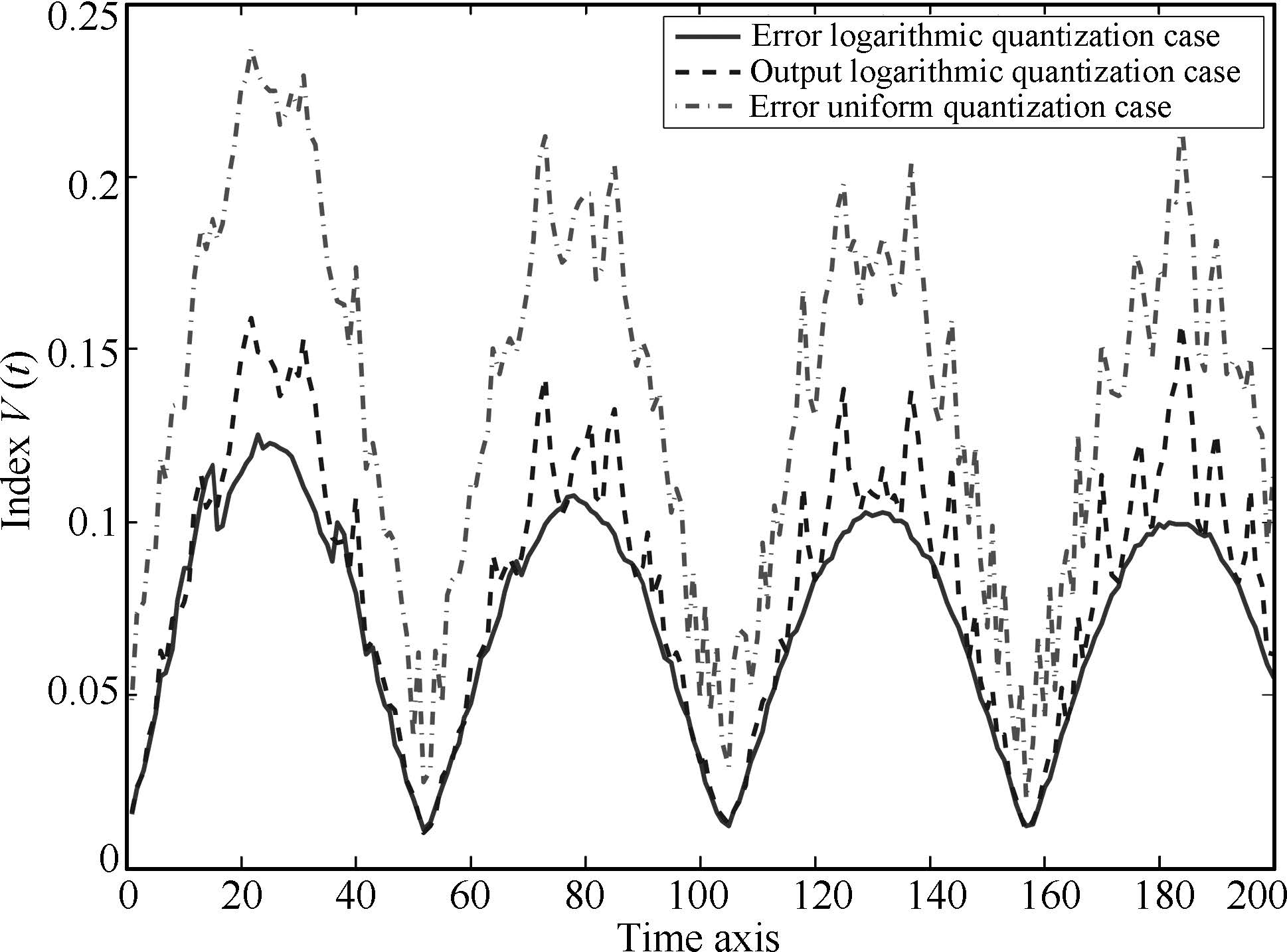
For brevity of expression,in this section,the update laws (6), (18) and (19) are called error logarithmic quantization law (ELQL),output logarithmic quantization law (OLQL) and error uniform quantization law (EUQL),respectively.

A.Linear Case

Consider the following linear system with random noises

$\begin{gathered} {x_k}(t + 1) = \left[{\begin{array}{*{20}{c}} { - 0.8 + 0.02\sin t}&{ - 0.22} \\ 1&0 \end{array}} \right]{x_k}(t) \hfill \\ \quad + \left[{\begin{array}{*{20}{c}} {0.5} \\ {1 - 0.05\cos (t/10)} \end{array}} \right]{u_k}(t) \hfill \\ \quad + {w_k}(t + 1),\hfill \\ {y_k}(t) = \left[{\begin{array}{*{20}{c}} 1&{0.5 + 0.5{{\text{e}}^{ - t}}} \end{array}} \right]{x_k}(t) + {v_k}(t),\hfill \\ \end{gathered}$

(20)

where $w_k(t)=[w_k^{(1)}(t),w_k^{(2)}(t)]^{\rm T}$ and $w_k^{(1)}(t)\sim {\rm N}(0,0.1^2)$,$w_k^{(2)}(t)\sim {\rm N}(0,0.1^2)$,$v_k(t)\sim {\rm N}(0,0.1^2)$,$\forall k,t$.

The desired tracking reference is given as $y_d(t)=5\sin(4t/25)+3\sin(2t/25)$,$t\in [0,100]$. Thus the initial desired state is $x_d(0)=0$. Let us set the initial state as $x_k(0)\sim {\rm N}(0,0.1^2)$ according to A4. The initial input is given as $u_0(t)=0$,$\forall t$.

The parameters of the logarithmic quantizer adopted in this section are selected $z_0=20$ and $\mu=0.7$. Thus it is a rough quantizer in a certain sense. The parameters of the uniform quantizer is $\nu=2/3$. The learning gain $a_k$ is chosen as $a_k=2.3/k$ satisfying the requirements in Theorem 1. The algorithm is performed for 100 iterations.

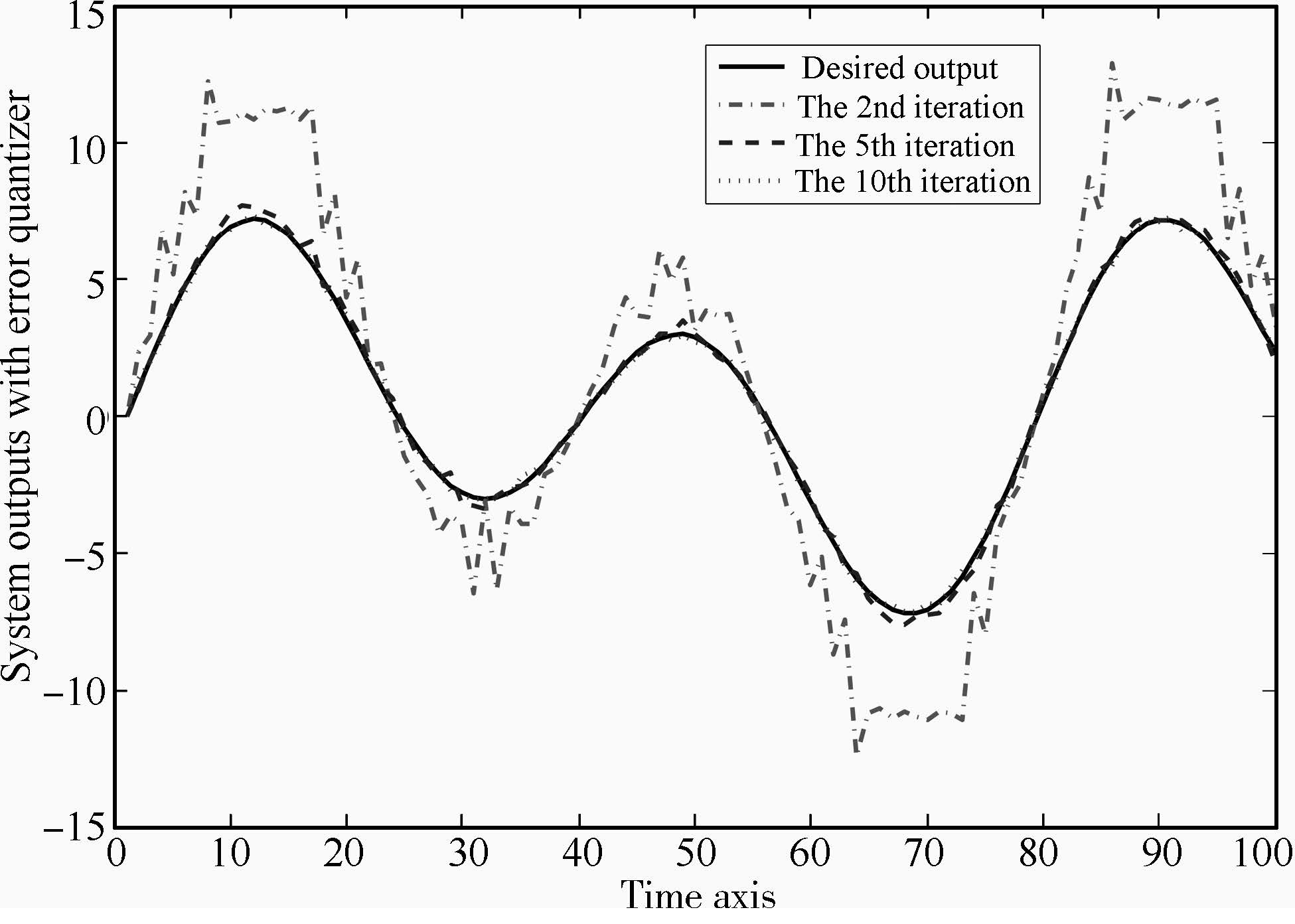
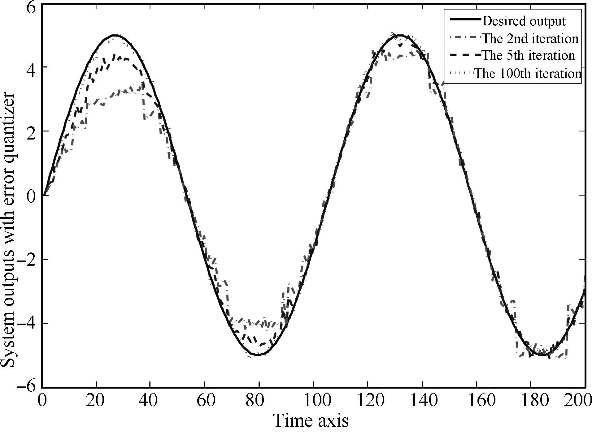
The tracking performance at the 2nd,5th,and 100th iterations is shown in Fig.2. One could find that the output tracking performance at the 5th iteration is acceptable while at the 100th iteration almost coincides with the desired reference. Thus the proposed algorithm is quite effective for iterative learning tracking.

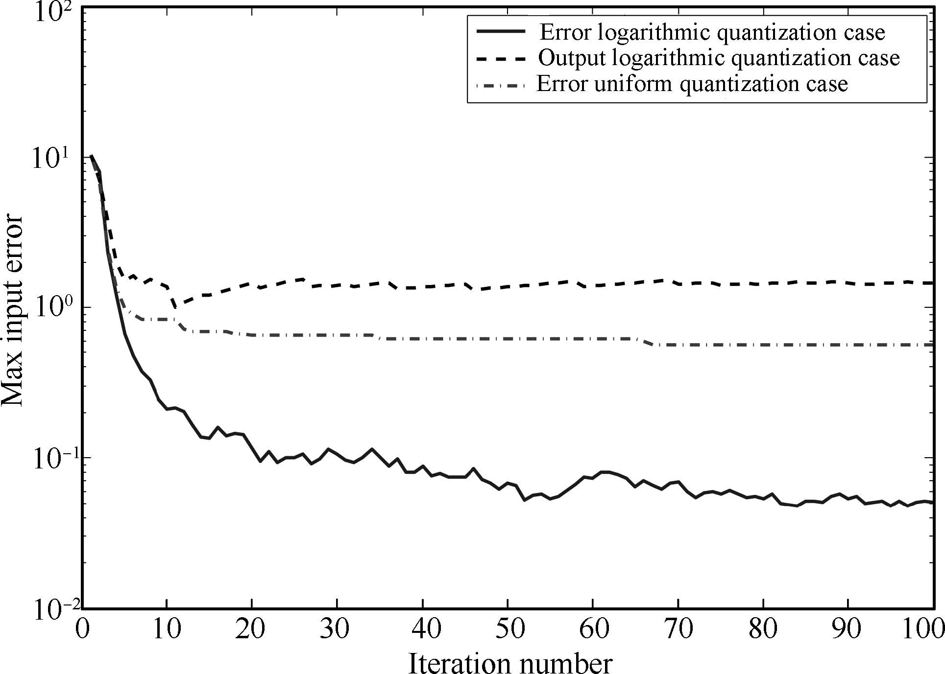
In addition,Fig.3 shows the convergence of input sequences for ELQL,OLQL and EUQL cases,where the solid,dash,and dash-dotted lines denote the maximal errors $\max_t|u_d(t)-u_k(t)|$,between the generated input and the desired input for ELQL,OLQL,and EUQL cases,respectively. The figure is plotted in logarithmic form to be more illustrative. Thus,to show the convergence of input,it should be illustrated that these errors converge to zero. From the figure,one could find that the ELQL case keeps a downward trend as iteration number increases,while the other two cases converge to nonzero values quickly. Besides,the maximal error of ELQL case is much smaller than those of the other two cases. Thus the ELQL case has a much better performance than the other two cases.

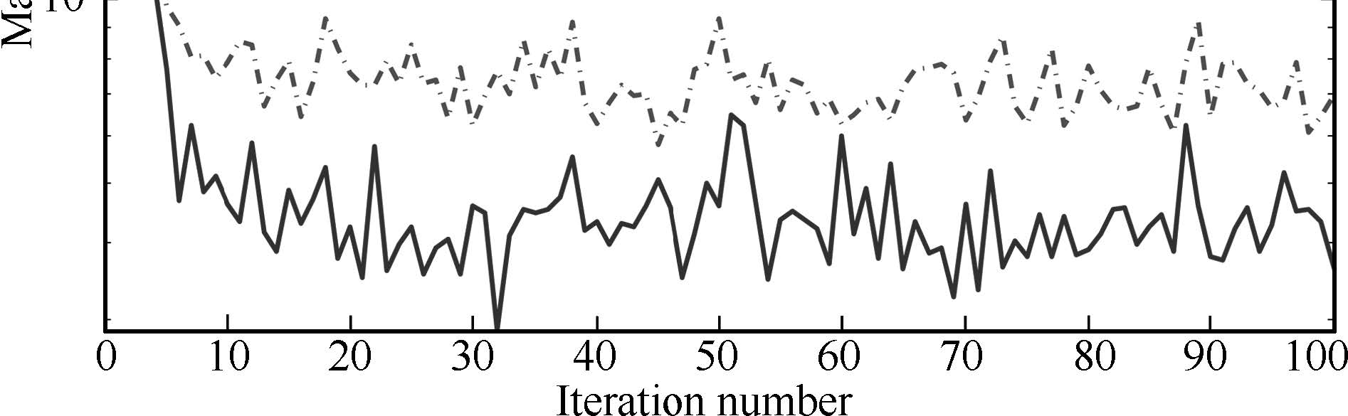
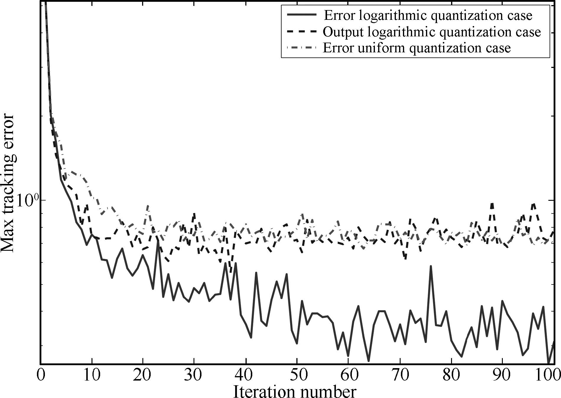
The maximal tracking errors,$\max_t|e_k(t)|$,are shown in Fig.4,which further verifies the effectiveness. As one could see from the figure,the ELQL case,denoted by solid line,behaves better than the OLQL case,denoted by dash line and the EUQL case, denoted by dash-dotted line. This is because the quantization error is reduced as the tracking error goes to zero in the ELQL case while the quantization error is large when the desired reference value is large in the OLQL case and the quantization error would not decrease further if the tracking error has come into the smallest bound of the uniform quantizer in the EUQL case. It should be pointed out that the maximal tracking error could not converge to zero due to the existence of random noises.

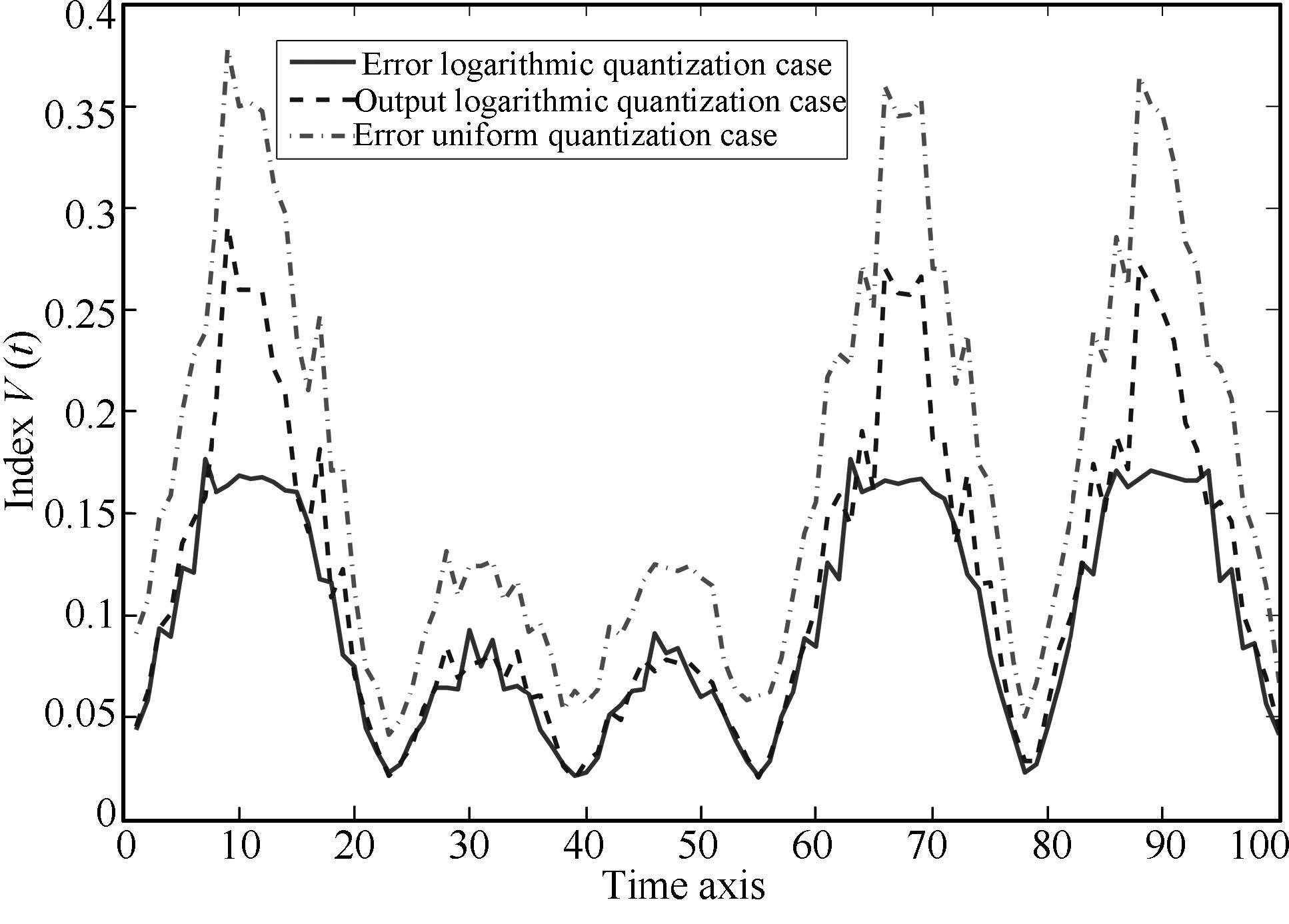
To make a more intuitive comparison on the performance of ELQL, OLQL,and EUQL cases,the tracking index $V(t)$ is computed for 100 iterations and shown in Fig.5. The index values in the ELQL case are much smaller than those in OLQL and EUQL cases,which coincide with the fact that the averaged tracking error in the ELQL case is mainly generated by stochastic noises while the average error in OLQL and EUQL cases are caused by both quantization errors and stochastic noises.

Additionally,some comments are given as follows. In the OLQL case,the output is quantized and thus the quantization error might be large if the output is large by noticing the properties of selected logarithmic quantizer. Consequently,the quantizer should be denser to make a more accurate tracking. That is,the parameter $\mu$ should be a bit larger. As a matter of fact,we further make simulations for the case $\mu=0.9$ and it is seen that the differences between the OLQL case and the ELQL case are much smaller. Therefore,the OLQL depends more on the quantizer while the ELQL could behave well even the quantization is rough.

As mentioned in Remark 3,the learning gain parameter $a_k$ needs to guarantee convergence and suppress noise. Thus $\{a_k\}$ has to satisfy the conditions given in the theorems. It is obvious that $a_k=a/k$ meets these requirements,where $a>0$ is a suitable constant. For practical applications,the constant $a$ should be set appropriately large in order to make a fast convergence but also not too large to lead to a bad tracking performance.

B.Nonlinear Case

For the nonlinear case,let us consider the following system

$\begin{array}{*{20}{l}} {{x_k}(t + 1) = }&{\left[{\begin{array}{*{20}{c}} { - 0.75\sin (x_k^{(1)}(t))} \\ { - 0.5\cos (x_k^{(2)}(t))} \end{array}} \right]} \\ {}&{ + \left[{\begin{array}{*{20}{c}} {0.5 + 0.1\cos (x_k^{(1)}(t)/5)} \\ 1 \end{array}} \right]{u_k}(t),} \\ {{y_k}(t) = }&{[0.10.02{t^{1/3}}]{x_k}(t) + {v_k}(t),} \end{array}$

(21)

where $x_k(t)=[x_k^{(1)}(t),x_k^{(2)}(t)]^{\rm T}$. Noise $v_k(t)$ is same as in the linear case.

The desired tracking reference is given as $y_d(t)=5\sin(3t/50)$, $t\in [0,200]$. The initial desired state is set $x_k(0)=x_d(0)=0$. The initial input is $u_0(t)=0$,$\forall t$.

The parameters of quantizers are the same as in the linear case. The learning gain $a_k$ is $a_k=6.5/k$. The algorithm is performed for 100 iterations.

Fig.6 shows the tracking performance at the 2nd,5th,and 100th iteration. It is seen that the output at the 100th iteration is satisfactory. The convergence of input sequence for both ELQL,OLQL and EUQL cases are provided in Fig.7. Here the input error is caused by the coupling of nonlinearities and stochastic noises. In addition,the decreasing gain $a_k$ also makes a slow improvement in input. In other words,much more iterations are needed for further improvements in input. However,it should be noted that the maximal input error for the ELQL case keeps decreasing along iteration axis, which is apparently different from the other two cases.

The maximal tracking error,$\max_t|e_k(t)|$,along iteration is shown in Fig.8 while the averaged index value is computed in Fig.9,respectively. Similar conclusions to the linear case could be derived.

Ⅵ. Concluding Remarks

In this paper,the ILC problem for both linear and nonlinear discrete-time systems with stochastic noises is considered under networked control system scheme. An update law is built based on quantized error information,which is generated from the plant side by comparing and quantizing using a logarithmic quantizer. In this case,the stochastic noises and quantization errors are coupled in the transmitted data. A decreasing learning gain is introduced to the algorithm and it is proved that the input sequence would converge to the optimal input under averaged tracking performance index. Two illustrative simulations are provided for both linear and nonlinear systems and the results coincide with theoretical analysis. For further research,it is of great interest to consider relaxations on the selection of quantizer.

APPENDIX A

PROOF OF LEMMA 1

For simplicity of expression,denote $\delta x_k(t):= x_d(t)-x_k(t)$and $\delta u_k(t):= u_d(t)-u_k(t)$. From (1) and (4),we have: $\delta {x_k}(t + 1) = A(t)\delta {x_k}(t) + B(t)\delta {u_k}(t) - {w_k}(t + 1),$ and recursively this leads to $\delta {x_k}(t + 1) = \sum\limits_{i = 1}^{t + 1} {\left( {\prod\limits_{l = i}^t A (l)} \right)} B(i - 1)\delta {u_k}(i - 1) - \sum\limits_{i = 0}^{t + 1} {\left( {\prod\limits_{l = i}^t A (l)} \right)} {w_k}(i),$ where $\prod_{l=i}^{j}A(l):= A(j)A(j-1)... A(i)$,$j\geq i$ and $\prod_{l=i}^{j}A(l)=I$,$j<i$. Thereby $\begin{gathered} {y_d}(t + 1) - {y_k}(t + 1) = C(t + 1)\delta {x_k}(t + 1) - {v_k}(t + 1) \hfill \\ = {\phi _k}(t + 1) + {\varphi _k}(t + 1) - {v_k}(t + 1),\hfill \\ \end{gathered} $ where $\begin{gathered} {\phi _k}(t + 1) = C(t + 1)\sum\limits_{i = 1}^{t + 1} {\left( {\prod\limits_{l = i}^t A (l)} \right)} B(i - 1)\delta {u_k}(i - 1),\hfill \\ {\varphi _k}(t + 1) = C(t + 1)\sum\limits_{i = 0}^{t + 1} {\left( {\prod\limits_{l = i}^t A (l)} \right)} {w_k}(i). \hfill \\ \end{gathered} $ By A3 and A4 and noticing that $u_k(i)\in\mathcal{F}_{k-1}$, $i=0,1,...,t$,it is clear that $\phi_k(t+1)$, $\varphi_k(t+1)$,and $v_k(t+1)$ are mutually independent.

It is noticed that

$\begin{gathered} \sum\limits_{k = 1}^n {{\phi _k}} (t)({\varphi _k}(t) - {v_k}(t)) = O\left( {{{\left( {\sum\limits_{k = 1}^n {{\phi _k}(t){^2}} } \right)}^{\frac{1}{2} + \gamma }}} \right),\hfill \\ \qquad \qquad \qquad \qquad \forall \gamma > 0,\hfill \\ \end{gathered}$

(A1)

$\begin{gathered} \sum\limits_{k = 1}^n {{\varphi _k}} (t){v_k}(t) = O\left( {{{\left( {\sum\limits_{k = 1}^n {{v_k}(} t){^2}} \right)}^{\frac{1}{2} + \gamma }}} \right),\hfill \\ \qquad \qquad \qquad \qquad \forall \gamma > 0. \hfill \\ \end{gathered}$

(A2)

Consequently, $\begin{gathered} \mathop {\lim \sup }\limits_{n \to \infty } \frac{1}{n}\sum\limits_{k = 1}^n {{y_d}(} t + 1) - {y_k}(t + 1){^2} \hfill \\ = \mathop {\lim \sup }\limits_{n \to \infty } \frac{1}{n}\sum\limits_{k = 1}^n {{\phi _k}(t + 1){^2}} \hfill \\ \end{gathered} $ $\begin{align} & ~+\underset{n\to \infty }{\mathop{\lim \sup }}\,\frac{1}{n}\sum\limits_{k=1}^{n}{\|{{\varphi }_{k}}(t+1){{\|}^{2}}} \\ & +\underset{n\to \infty }{\mathop{\lim \sup }}\,\frac{1}{n}\sum\limits_{k=1}^{n}{\|{{v}_{k}}(}t+1){{\|}^{2}}~ \\ & ~=\underset{n\to \infty }{\mathop{\lim \sup }}\,\frac{1}{n}\sum\limits_{k=1}^{n}{\|{{\phi }_{k}}(t+1){{\|}^{2}}} \\ & +\text{tr}[C(t+1)\sum\limits_{i=0}^{t+1}{\left( \prod\limits_{l=i}^{t}{A}(l) \right)}R_{w}^{t}~ \\ & ~\times {{\left( \prod\limits_{l=i}^{t}{A}(l) \right)}^{\text{T}}}{{C}^{\text{T}}}(t+1)+R_{v}^{t+1}],\\ \end{align}$ where the last term is independent of the control.

Therefore,the tracking index (2) is minimized if the first term of last equation,i.e., $\limsup_{n\rightarrow\infty}\frac{1}{n}\sum_{k=1}^n\|\phi_k(t+1)\|^2$, equals zero. It is clear that the condition is satisfied if $u_k(t)\rightarrow u_d(t)$ as $k\rightarrow\infty$.

APPENDIX B

PROOF OF THEOREM 1

Denote $\delta x_k(t):= x_d(t)-x_k(t)$ and $\delta u_k(t):= u_d(t)-u_k(t)$. From (6) we have

$\delta {{u}_{k+1}}(t)=\delta {{u}_{k}}(t)-{{a}_{k}}Q({{e}_{k}}(t+1)).$

(A3)

Substituting (9) into last equation leads to

$\delta {{u}_{k+1}}(t)=\delta {{u}_{k}}(t)-{{a}_{k}}(1+\Delta {{e}_{k}}(t+1)){{e}_{k}}(t+1),$

(A4)

where $|\eta_k^t|\leq \zeta<1$,$\forall t$. Thus,we have $\begin{align} & \delta {{u}_{k+1}}(t)=\delta {{u}_{k}}(t)-{{a}_{k}}(1+\eta _{k}^{t+1}){{e}_{k}}(t+1) \\ & =\delta {{u}_{k}}(t)-{{a}_{k}}(1+\eta _{k}^{t+1}) \\ & (C(t+1)A(t)\delta {{x}_{k}}(t)n+{{C}^{+}}B(t)\delta {{u}_{k}}(t))n \\ & +{{a}_{k}}(1+\eta _{k}^{t+1})({{v}_{k}}(t+1)+C(t+1){{w}_{k}}(t+1))n \\ & =(1-{{a}_{k}}(1+\eta _{k}^{t+1}){{C}^{+}}B(t))\delta {{u}_{k}}(t)n- \\ & {{a}_{k}}(1+\eta _{k}^{t+1})C(t+1)A(t)\delta {{x}_{k}}(t)n+ \\ & {{a}_{k}}(1+\eta _{k}^{t+1})({{v}_{k}}(t+1)+C(t+1){{w}_{k}}(t+1))n \\ & =(1-{{a}_{k}}(1+\eta _{k}^{t+1}){{C}^{+}}B(t))\delta {{u}_{k}}(t)n- \\ & {{a}_{k}}(1+\eta _{k}^{t+1})C(t+1)n\times \sum\limits_{i=1}^{t}{\left( \prod\limits_{l=i}^{t}{A}(l) \right)} \\ & B(i-1)\delta u(i-1)+{{a}_{k}}(1+\eta _{k}^{t+1})({{v}_{k}}(t+1) \\ & +C(t+1)\sum\limits_{i=0}^{t+1}{\left( \prod\limits_{l=i}^{t}{A}(l) \right)}{{w}_{k}}(i)). \\ \end{align}$ Define $H=\left[\begin{matrix} {{C}^{+}}B(0) & 0 & ... & 0 \\ C(2)A(1)B(0) & {{C}^{+}}B(1) & ... & 0 \\ \vdots & \vdots & \ddots & \vdots \\ C(N)\prod\limits_{l=1}^{N-1}{A}(l)B(0) & ... & ... & {{C}^{+}}B(N-1) \\ \end{matrix} \right],$ and $\Gamma_k=\left[\begin{array}{cccc} 1+\eta_k^1&0&...&0\\ 0&1+\eta_k^2&...&0\\ \vdots&\vdots&\ddots&\vdots\\ 0&0&...&1+\eta_k^N \end{array}\right].$

Then stack the input into a vector $\delta U_k=[\delta u_k(0),\delta u_k(1),...,\delta u_k(N-1)]^{\rm T}$ and the noise term into $\xi_k=\left[\begin{array}{c} C(1)\sum\limits_{i=0}^{1}\left(\prod\limits_{l=i}^0A(l)\right)w_k(i)+v_k(1)\\ C(2)\sum\limits_{i=0}^{2}\left(\prod\limits_{l=i}^1A(l)\right)w_k(i)+v_k(2)\\ \vdots\\ C(N)\sum\limits_{i=0}^{N}\left(\prod\limits_{l=i}^{N-1}A(l)\right)w_k(i)+v_k(N) \end{array}\right].$ Now from the above expressions we have:

$\delta {{U}_{k+1}}=(I-{{a}_{k}}{{\Gamma }_{k}}H)\delta {{U}_{k}}+{{a}_{k}}{{\Gamma }_{k}}{{\xi }_{k}},$

(A5)

where $I$ denotes the unit matrix with appropriate dimension.

Noticing that $\Gamma_k$ is a diagonal matrix and $H$ is a lower triangular matrix,it is obvious that $\Gamma_kH$ also is a lower triangular matrix,thus,the eigenvalues of $\Gamma_kH$ are its diagonal elements. By the definition of $\Gamma_k$ and $H$ it is clear that the eigenvalues of $\Gamma_kH$ are $(1+\eta_k^1)C^+B(0)$,$...$,$(1+\eta_k^N)C^+B(N-1)$. Since $|\eta_k^t|<1$,it is evident$1+\eta_k^t>0$,$\forall t$. Combining with A1,we have that $(1+\eta_k^t)C^+B(t-1)$ is positive,$1\leq t\leq N$. In addition, $\eta_k^t>-\zeta=-(1-\mu)/(1+\mu)$,thus $1+\eta_k^t>2\mu/(1+\mu)$. Therefore,there is a lower bound for each eigenvalue of $\Gamma_kH$. This means that there is a positive definite matrix $P$ such that $(\Gamma_kH)^{\rm T}P+P\Gamma_kH\geq I.$ Set

${{\Phi }_{k,j}}=(I-{{a}_{k}}{{\Gamma }_{k}}H)...(I-{{a}_{j}}{{\Gamma }_{j}}H),\quad \forall k\ge j.$

(A6)

Now we first give an estimation on the growth of $\Phi_{k,j}$. To be specific,there are constants $c_0>0$ and $c>0$ such that

$\|{{\Phi }_{k,j}}\|\le {{c}_{0}}\exp \left[-c\sum\limits_{i=j}^{k}{{{a}_{i}}} \right],\forall k\ge j,\forall j\ge 0.$

(A7)

It is noticed that $\begin{align} & \Phi _{k,j}^{\text{T}}P{{\Phi }_{k,j}}=\Phi _{k-1,j}^{\text{T}}{{(I-{{a}_{k}}{{\Gamma }_{k}}H)}^{\text{T}}}P(I-{{a}_{k}}{{\Gamma }_{k}}H){{\Phi }_{k-1,j}} \\ & =\Phi _{k-1,j}^{\text{T}}(P+a_{k}^{2}{{H}^{\text{T}}}\Gamma _{k}^{\text{T}}P{{\Gamma }_{k}}H-{{a}_{k}}{{H}^{\text{T}}}\Gamma _{k}^{\text{T}}P-{{a}_{k}}P{{\Gamma }_{k}}H){{\Phi }_{k-1,j}} \\ & \le \Phi _{k-1,j}^{\text{T}}(P+a_{k}^{2}{{H}^{\text{T}}}\Gamma _{k}^{\text{T}}P{{\Gamma }_{k}}H-{{a}_{k}}I){{\Phi }_{k-1,j}} \\ & =\Phi _{k-1,j}^{\text{T}}{{P}^{\frac{1}{2}}}(I-{{a}_{k}}{{P}^{-1}}+a_{k}^{2}{{P}^{-\frac{1}{2}}}{{H}^{\text{T}}}\Gamma _{k}^{\text{T}}P{{\Gamma }_{k}}H{{P}^{-\frac{1}{2}}}){{P}^{\frac{1}{2}}}{{\Phi }_{k-1,j}}. \\ \end{align}$ Without loss of generality we may assume for $j_0$ to be large enough such that $\forall j\geq j_0$

$\begin{align} & \|I-{{a}_{k}}{{P}^{-1}}+a_{k}^{2}{{P}^{-\frac{1}{2}}}{{H}^{\text{T}}}\Gamma _{k}^{\text{T}}P{{\Gamma }_{k}}H{{P}^{-\frac{1}{2}}}\| \\ & \le 1-2c{{a}_{k}}<{{\text{e}}^{-2c{{a}_{k}}}},\\ \end{align}$

(A8)

for some constant $c>0$,where the first inequality is because $a_k\rightarrow0$,$P^{-1}>0$ and $k\geq j$ according to (A6), while the second inequality is elementary. This leads to $\Phi_{k,j}^{\rm T}P\Phi_{k,j}\leq \left(\exp\left(-2c\sum_{i=j}^ka_i\right)\right)I,$ and hence there is constant $c_0>0$ such that the estimation (A7) is valid for $j\geq j_0$ to be large enough. Further,$j_0$ is finite,thus with suitable selection of $c_0>0$ and $c>0$ the estimation (A7) also holds for any $k\geq j$.

Comparing with Lemma 3.3.1 in ^[13],it is seen that the rest steps could be carried out along the lines of the proof of Lemma 3.3.1 in ^[13] as long as we show that $\sum_{k=1}^{\infty}a_k\Gamma_k\xi_k<\infty$. It should be pointed out that the diagonal elements of $\Gamma_k$,$1+\eta_k^t$,depend on $e_k(t)$,and consequently depend on $u_k(t-1)$,$\forall t$. In other words,the term $\Gamma_k$ is dependent on $\delta U_k$. That is,$\{\Gamma_k\xi_k\}$ is not an independent sequence.

However,by the definition of ${F_k}$ and $\delta U_k$, and assumptions A3-A4,it is found that $\Gamma_k$ is independent of $\xi_k$. Further,${\rm E}(\Gamma_k\xi_k|\mathcal{F}_{k-1})=\Gamma_k{\rm E}(\xi_k|\mathcal{F}_{k-1})=0$. In addition,$\{a_k\}$ is a prior given sequence. Thus,$(a_k\Gamma_k\xi_k,\mathcal{F}_k)$ is a martingale difference sequence.

Noticing $|\eta_k^t|<1$,thus $\Gamma_k$ is bounded,i.e., $\|\Gamma_k\|^2<c_1$ with suitable $c_1>0$. Then,we have $\sum_{k=1}^{\infty}{\rm E}\|a_k\Gamma_k\xi_k\|^2 \leq c_1 \sum_{k=1}^{\infty}a_k^2{\rm E}\|\xi_k\|^2 \leq c_1c_2 \sum_{k=1}^{\infty}a_k^2<\infty,$ where $c_2>0$is a suitable constant which depends on $R_w^t$, $R_v^t$,and $R_0$. By martingale difference convergence theorem it is evident that $\sum_{k=1}^{\infty}a_k\Gamma_k\xi_k<\infty$.

APPENDIX C

PROOF OF LEMMA 2

The proof of this lemma can be carried out by induction along the time axis $t$. From (10) and (11) it is noted that

$\begin{array}{*{35}{l}} \delta {{x}_{k}}(t+1)= & {{f}_{d}}(t)-{{f}_{k}}(t)+{{B}_{d}}(t){{u}_{d}}(t)-{{B}_{k}}(t){{u}_{k}}(t) \\ = & \delta {{f}_{k}}(t)+\delta {{B}_{k}}(t){{u}_{d}}(t)+{{B}_{k}}(t)\delta {{u}_{k}}(t). \\ \end{array}$

(A9)

First,let us consider $t=0$. From A6 and A8,we have $\begin{align} & \delta {{f}_{k}}(0)={{f}_{d}}(0)-{{f}_{k}}(0)\to 0,\\ & \delta {{B}_{k}}(0)={{B}_{d}}(0)-{{B}_{k}}(0)\to 0. \\ \end{align}$ This further leads to that the first two terms at the right-hand side of (A9) tend to zero as $k\rightarrow\infty$. Since $\|B_k(0)\|=\|B_d(0)\|+\|\delta B_k(0)\|$,it follows that $B_k(0)$ is bounded. Thus,if $\delta u_k(0)\rightarrow0$,the third term at the right-hand side of (A9) also tends to zero. This further implies that $\delta x_k(1)\rightarrow0$ and then by A6 gain,$\delta f_k(1)\rightarrow0$ and $\delta B_k(1)\rightarrow0$. That is,the conclusion is valid for the initial time instance $t=0$.

Inductively,let us now assume that the conclusion of the lemma is true for $s=0,1,...,t-1$. It suffices to show that the conclusion is valid for $t$,i.e.,$\delta x_k(t+1)\rightarrow0$, $\delta f_k(t+1)\rightarrow0$,and $\delta B_k(t+1)\rightarrow0$. This could be done by similar steps as above.