 2016, Vol.3


2. Institute of Intelligent Machines, Chinese Academy of Sciences, 230031 Hefei, China;
3. Department of Chemistry, Princeton University, Princeton, New Jersey 08544, USA
During the last three decades,people have made
considerable achievements on the research of quantum information
processing
[1, 2, 3, 4, 5, 6]. Practical quantum information processing still
confronts with some important technical difficulties,such as the
laser noise,environmental decoherence effects and quantum
measurement. Quantum measurement is generally considered as a
deleterious factor toward the manipulation of quantum
dynamics[7, 8, 9, 10],which induces the disappearance of coherence of
the system's state irreversibly. However,recent studies have shown
that both the outcome and back-action from quantum measurements
could be used to control the quantum systems[11, 12, 13, 14]. In
standard closed-loop optimal quantum control,the outcomes of the
measurements are used by a learning algorithm to optimize the
coherent control field Projective measurement is the most generally used quantum
observations. The manipulation of quantum dynamics driven by the
quantum projective measurements is explored theoretically
This paper explores some deep characteristics of the manipulation between eigenstates of a two-level system by optimal measurements. We consider a two-level system measured by a sequence of non-selective projection operators. Measurements are designed and performed instantaneously with a fixed frequency,so that the system in each interval can be seen as a closed quantum system. The measurement unavoidably affects the quantum state,so as to drive the system to the target state. We investigate three cases of the manipulations under the optimal measurements. The first is the optimal measurements itself,which is the ideal case. Then we further explore the effect of free evolution of the system to the manipulation. In the end,the performances of manipulation of the optimal measurements in the case with the external control fields are studied in order to compensate for the effect of the free evolution. Numerical simulations of the three cases are conducted to verify the enhanced effectiveness.
The rest of the paper is organized as follows: In Section Ⅱ,the concepts of optimal measurement-based control are presented. The cases with the free evolution and the external control fields are analyzed and discussed. The analytical solutions are derived for three cases. In Section Ⅲ,numerical simulations for three cases are conducted. The characteristics are discussed,and the optimal parameters of manipulations are obtained. A brief conclusion is in Section IV.
II. QUANTUM CONTROL BY OPTIMAL MEASUREMENTS A. Optimal Control with Projective MeasurementsConsider a two-level quantum system,with $\rho $ being the density operator of the system. Suppose an instantaneous projective measurement be performed on the state,and the state density operator after the measurement will be $\rho '$:
| $ \rho ' = P\rho P + (I-P)\rho (I-P) = \rho-[P,[P,\rho]], $ | (1) |
where $I $ is the identity operator and $P $ is the projection operator. The instantaneous measurement is characterized by the set of projection operators $\{ P,I-P\}$ .
One can see from (1) that an important characteristic of the quantum measurements is to generally change the quantum state. However,on the other hand,quantum measurements can also be employed to actively control the quantum system dynamics by means of such a characteristic.
Our research objective is to manipulate the state in a two-level system by instantaneous projective measurements from the initial state ${\rho _0} = \left| 0 \right\rangle \left\langle 0 \right|$ to the target state ${\rho _f} = \left| 1 \right\rangle \left\langle 1 \right| $ . The projection operators are specified by the operators
| $ {P_k} = \left| {{\psi _k}} \right\rangle \langle {\psi _k}|, $ | (2) |
| $ \left| {{\psi _k}} \right\rangle = \cos \frac{{{\alpha _k}}}{2}\left| 0 \right\rangle + {{\rm{e}}^{i{\theta _k}}}\sin \frac{{{\alpha _k}}}{2}\left| 1 \right\rangle , $ | (3) |
where $\left| {{\psi _k}} \right\rangle $ is the basis vector of ${P_k}$ ( $k = 1,...,m $ ), ${\alpha _k}$ and ${\theta _k} $ are parameters of ${P_k}$ and limited to the ranges: $-\frac{\pi }{2} \le \frac{{{\alpha _k}}}{2} \le \frac{\pi }{2} $ , $ 0 \le {\theta _k} < \pi $ . Let ${\rho _k} $ be the state after the $k $-th measurement and
| $ {\rho _k} = {\rho _{k-1}}-[{P_k},[{P_k},{\rho _{k-1}}]], $ | (4) |
where ${\rho _{k-1}} $ is the state after the $(k-1) $ -th measurement and ${\rho _m} $ is the final state. Equation (4) is an iterative equation of the transfer. Given a set of projection operators $\{ {P_1},...,{P_m}\} $ ,one can easily calculate ${\rho _m} $. The fidelity between the initial state ${\rho _m} $ and the target state ${\rho _f} $ is defined as
| $ F({\rho _m},{\rho _f}) = {\left[{{\mathop{\rm tr}\nolimits} (\sqrt {\sqrt {{\rho _m}} {\rho _f}\sqrt {{\rho _m}} } )} \right]^2}. $ | (5) |
The analytical solution of
$F({\rho _m},{\rho _f})$
reaches maximum
value when the manipulation from
${\rho _m}$
to
${\rho _m}$
is
optimized
| $ {\theta _1} = {\theta _2} = \cdot \cdot \cdot = {\theta _k} = 0, $ | (6) |
| $ {\theta _1} = {\theta _2} = \cdot \cdot \cdot = {\theta _k} = 0, $ | (7) |
where ${\theta _k}$ and ${\alpha _k}$ ( $k = 1,...,m$ ) are the parameters of the projection operators. Substituting (6)-(7) into (3) and (2),one can obtain the corresponding optimal projection operators,and can easily derive the corresponding fidelity as
| $ {F_m} = \frac{1}{2}\left[{1 + {{\left( {\cos \frac{\pi }{{m + 1}}} \right)}^{m + 1}}} \right], $ | (8) |
where ${F_m}$ is the optimal value of $F({\rho _m},{\rho _f})$ . Equation (8) is the expression for the the optimal fidelity ${F_m}$ with the corresponding measurement time $m$ .
It is easy to see from (8) that ${F_m}$ increases monotonically with $m$ increasing. The minimum value of ${F_m}$ is 0.5 when $m = 1$ . The maximum value of ${F_m}$ approaches $100 \% $ when $m$ tends to infinity. Therefore,the value of ${F_m}$ is in the range of $[0.5,1)$. In other words,when measuring infinite times to a quantum system,we can realize $100 \% $ transferring from an initial state to the target state,which is the so-called ``quantum anti-Zeno effect''.
B.Optimal Measurement-based Control with Free Evolution of the SystemIn fact,there is always free evolution in a quantum system. So a more realistic measurement-based control should consider the free evolution of the system itself. In this section we analyze the effect of free evolution to the optimal measurement-based control.
Suppose the instantaneous projective measurements change the state instantaneously and do not affect the characteristics of the system. The time interval of two measurements is fixed as $\Delta t $ . The system dynamics with free evolution is
| $ {\dot \rho _k}(t) =-i[{H_0},{\rho _k}(t)], $ | (9) |
where, ${\rho _k}(t)$ is the state in the interval between the $k$ -th and $(k+1)$ -th measurement, $k = 1,...,m$ , $t \in [0,\Delta t]$ . ${H_0}$ is the free Hamiltonian:
| $ {{H}_{0}}={{\sigma }_{z}}=\left| \begin{matrix} 1 & 0 \\ 0 & -1 \\ \end{matrix} \right|, $ | (10) |
where ${\sigma _z}$ is Pauli operator. The solution of (9) is
| $ {\rho _k}(t) = {{\rm e}^{-i{H_0}t}}{\rho _k}(0){{\rm e}^{i{H_0}t}}. $ | (11) |
Since the quantum state changes with the free evolution,the iterative equation of the transfer is different from (4). Substituting (10)-(11) into (4),one can obtain the iterative equation with the free evolution:
| $ {\rho _k}(0) = {\rho _{k-1}}(\Delta t)-[{P_k},[{P_k},{\rho _{k -1}}(\Delta t)]], $ | (12) |
in which ${\rho _{k-1}}(\Delta t)$ is defined in (11).
When the optimal measurement control is performed in the case with free evolution,the optimal fidelity between ${\rho _m}$ and ${\rho _f}$ becomes:
| $ \begin{align} \begin{array}{c} {F_m} = \displaystyle\frac{1}{2}\left[{1 + {C_m} \cdot \prod\limits_{k = 1}^m {\left( {{C_m}-2\sin {\alpha _k} \cdot \sin {\alpha _{k-1}} \cdot {{\sin }^2}(\Delta t)} \right)} } \right]\\ = \displaystyle\frac{1}{2}\left[{1 + {C_m} \cdot \prod\limits_{k = 1}^m {\left( {{C_m}-2{S_{mk}} \cdot {S_{m(k-1)}} \cdot {{\sin }^2}(\Delta t)} \right)} } \right], \end{array} \end{align} $ | (13) |
where ${C_m}$ , ${S_{mk}}$ and ${S_{m(k-1)}}$ represent $\cos (\frac{\pi }{{m + 1}})$ , $\sin (\frac{{k\pi }}{{m + 1}})$ and $\sin (\frac{{(k-1)\pi }}{{m + 1}})$ ,respectively. From (13),one can see that ${F_m}$ depends on $m$ and $\Delta t$ in the case with free evolution.
According to the symmetry of the trigonometric functions,it is easy to verify that when $\Delta t > 0$,for any $m$ there is the following inequality:
| $ \begin{align} {C_m} \cdot \prod\limits_{k = 1}^m {\left( {{C_m}-2{S_{mk}} \cdot {S_{m(k-1)}} \cdot {{\sin }^2}(\Delta t)} \right)} < {\left( {{C_m}} \right)^{m + 1}}. \end{align} $ | (14) |
It can be easily derived with (14) that the fidelity ${F_m}$ in (13) is smaller than that in (8). In summary,the free evolution of the system may decrease the effectiveness of the optimal fidelity,which gives a disturbance of the optimal measurement.
C.Optimal Measurement-based Control with External Control FieldsIn this section we will analyze the manipulation effect of the optimal measurement-based control by introducing the external control fields.
The dynamics of a two-level quantum system with free evolution and the external control fields can be expressed as:
| $ {\dot \rho _k}(t) =-i[H,{\rho _k}(t)], $ | (15) |
where $H = {H_0} + {u_x}{H_x} + {u_y}{H_y} + {u_z}{H_z}$ is the system Hamiltonian. ${H_0}$ is the free Hamiltonian, ${H_x}$ , ${H_y}$ and ${H_z}$ are the external control Hamiltonian with ${u_x}$ , ${u_y}$ and ${u_z}$ representing the corresponding control fields. The Hamiltonians are
| $ {H_0} = {\sigma _z},{H_x} = {\sigma _x},{H_y} = {\sigma _y},{H_z} = {\sigma _z}, $ | (16) |
where ${\sigma _x}$ , ${\sigma _y}$ and ${\sigma _z}$ are Pauli operators.
We need to design the shape of the control fields ${u_x}$ , ${u_y}$ and $/$ or ${u_z}$ in order to compensate for the effect of free evolution and increase the fidelity of optimal measurement control.
The solution of (15) is
| $ {\rho _k}(t) = {{\rm e}^{-iHt}}{\rho _k}(0){{\rm e}^{iHt}}, $ | (17) |
in which ${\rho _k}(0)$ is defined by the iteration equation of optimal measurement as:
| $ {\rho _k}(0) = {\rho _{k-1}}(\Delta t)-[{P_k},[{P_k},{\rho _{k -1}}(\Delta t)]]. $ | (18) |
It should be pointed out that the state ${\rho _{k-1}}(\Delta t)$ in (18) is calculated from (17),which is not the same as the state in (12).
Ⅲ. NUMERICAL SIMULATION AND THE CHARACTERISTIC ANALYSISIn this section,our tasks are to perform the simulation experiments,analyze the experimental results of manipulations, and determine the appropriate control fields designed. In the experiments,the initial and target states are both eigenstates, they are ${\rho _0} = \left| 0 \right\rangle \left\langle 0 \right|$ and ${\rho _f} = \left| 1 \right\rangle \left\langle 1 \right|$ ,respectively. Suppose the manipulation is achieved by $ $m$ $ times instantaneous projective measurements,and the projection operators $\left\{ {{P_1},{P_2},...,{P_m}} \right\}$ follow the optimal condition (2) and (3). The performance index of the fidelity is fixed as $95 \% $ .
A.Manipulation Between Eigenstates with Optimal MeasurementsThe first experiment is the manipulation between eigenstates with optimal measurements. The experimental results of optimal fidelities with $m$ being 1,5,10,30,46,100,500 and 1000,respectively, are shown in Table I,from which one can see that:
|
|
Table I OPTIMAL FIDELITY Fm OF THE STATE TRANSFER WITH DIFFERENT NUMBER OF MEASUREMENTS m |
1) When $m$ ,the optimal fidelity ${F_m}$ equals $50 \%$ . Because for one time's measurement,the state is just projected onto the maximum mixed state (Bloch vector $\vec O = (0,0,0)$ ).
2) As $m$ increases,the optimal fidelity reaches the given performance index of $95 \%$ for the first time when $m = 46$ and ${F_{46}} = 95.01 \%$ . So $m = 46$ is the minimum measurement number needed to achieve the desired performance index.
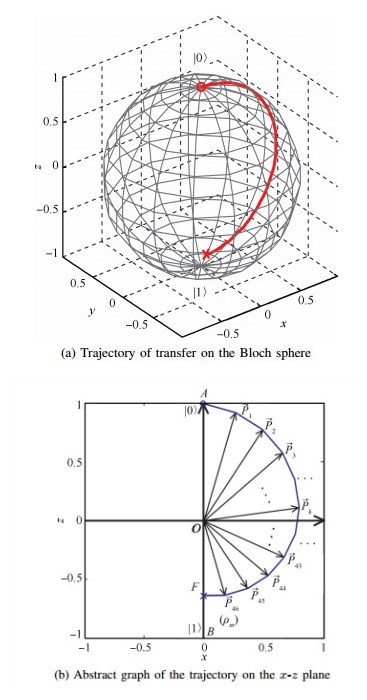
In order to do better analyses,the transfer trajectory of the system state is drawn on the Bloch Sphere as shown in Fig. 1,in which Fig. 1(a) is the transfer trajectory of the system state with $m = 46$ ,and Fig. 1(b) is the abstract graph of the trajectory on the $x$ - $z$ plane.

|
Download:
|
| Fig. 1 Transfer trajectory of the system state by projective measurements. | |
The vector of the initial state ${\rho _0}$ and the target state ${\rho _f}$ are ${\vec s_0} = (0,0,1)$ and ${\vec s_f} = (0,0,- 1)$ ,respectively. The red circle in Fig. 1 (a) represents the original state ${\rho _0}$ ,and the red cross represents the final state ${\rho _m}$ . One can see from Fig. 1 (a) that the trajectory is an approximate semi-circular,which is from the Bloch sphere's one pole to the other pole. The coordinate $y$ of the states in Fig. 1 (a) is 0,so it is obvious that the vectors of the states can be plotted on $x$ - $z$ plane as shown in Fig. 1 (b),where ${\vec P_i}$ represents the state ${\rho _i}$ . The angle between ${\vec P_i}$ and ${\vec P_i+1}$ is $\varphi = \pi /47$ ,which is defined in (7). Fig. 1 (b) indicates that each measurement rotates the preceding vector by the angle $\varphi = \pi /47$ clockwise and shortens its length by the factor $\cos \varphi $ . From Fig. 1 (b) one can easily derive the formula of optimal fidelity (7) by geometric analysis,which supplies an easier derivation method.
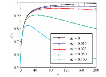
B.Manipulation Between Eigenstates with Free Evolution of the SystemIn this section,we will do the experiments of the manipulation between eigenstates with free evolution of the system. Let the time of measurement intervals be $\Delta t$ . To analyze the effect of $\Delta t$ on the performance,we investigate the ${F_m}$ as the function of $m$ with different values of $\Delta t$ . The optimal fidelity ${F_m}$ is calculated according to (13),and the experimental results are shown in Fig. 2,in which $\Delta t$ is set as five different values: $\Delta t = 0$ , $\Delta t = 0.015$ , $\Delta t = 0.023$ , $\Delta t = 0.05$ and $\Delta t = 0.1$ .

|
Download:
|
|
Fig. 2 The function of the optimal fidelity ${F_m}$ with different ∆ |
|
From Fig. 2 one can see that:
1) When $\Delta t = 0$ ,the transfer is equivalent to the experiment without free evolution. The function ${F_m}$ follows (8) and rises monotonically up to 1;
2) When $\Delta t > 0$ ,the functions ${F_m}$ are convex,and each function has a peak value $F_m^{(o)}$ ,which is the maximum fidelity.
In order to make the optimal fidelity ${F_m}$ with different $\Delta t$ meet the given performance,it is more meaningful to investigate the maximum fidelity $F_m^{(o)}$ . The experimental results of the maximum fidelities $F_m^{(o)}$ with different values of $\Delta t$ and the corresponding $m$ are shown in Table Ⅱ,from which one can see that: 1) When $\Delta t = 0.023$,the maximum fidelity is $F_{96}^{(o)} = 95.14 \% $ with $m = 96$; 2) When $\Delta t = 0.024$,the maximum fidelity is $F_{91}^{(o)} = 94.94 \% $ with $m = 91$. It can be concluded that on one hand, with the increment of $\Delta t$,the maximum value of ${F_m}$ decreases,as well as the corresponding measurement number $m$,on the other hand,when $\Delta t \ge 0.024$,the fidelity of optimal measurement control cannot reach $95 \%$ no matter how large the measurement number $m$ is. So we choose $\Delta t = 0.023$ as the optimal time of intervals,and in the later experiments of the paper $\Delta t$ is fixed as 0.023.
|
|
Table Ⅱ THE MAXIMUM FIDELITY $F_m^{(o)}$ OF DIFFERENT $\Delta t$ AND THE CORRESPONDING $m$ |
In this section,we will analyze the manipulation between eigenstates by optimal measurement control with the external control fields. The external control fields can be seen as a compensation for the effect of the free evolution of the system as well as a enhancement of control effect. In Section Ⅱ-C,we design the external control fields with three components: ${u_x}$, ${u_y}$ and$/$or ${u_z}$. In this section,we investigate the effectiveness of different control fields in two cases,one is to use only one control field and another is to use two control fields,and compare the performances in these two cases.
1) Case 1. Only one external control field applied
For simplicity,we just choose a constant field in this case. Because the free Hamiltonian ${H_0}$ is ${\sigma _z}$,we cannot only use ${u_z}$ on the system. We thought to use one of control fields ${u_x}$ or ${u_y}$. As the analysis in Fig. 1 (b),the state is projected onto the $x$-$z$ plane after each measurement, but the experimental results we did indicated that there is no evident compensation effectiveness by using control ${u_x}$. Therefore,a constant ${u_y}$ control field is used to drive the state rotate on the $x$-$z$ plane in the experiments. At the same time,the system is also affected by the measurements and free evolution.
The initial and target states in the experiments are the same as in Section Ⅱ-B,and the measurement interval time is set as $\Delta t = 0.023$. The control Hamiltonian is $H = {\sigma _z} + {u_y}{\sigma _y}$,and the system dynamics is:
| $ {\rho _k}(t) = {{\rm e}^{-i({\sigma _0} + {u_y}{\sigma _y})\Delta t}}{\rho _k}(0){{\rm e}^{i({\sigma _0} + {u_y}{\sigma _y})\Delta t}}. $ | (19) |
Using (18) and (19) alternately with the given initial state ${\rho_0}$ one can obtain the final state ${\rho _m}$.
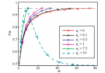
Fig. 3 shows the curves of $F_m$ of states manipulated by optimal measurements and an external control field in a two-level system, with the six different values of the control fields ${u_y}$: ${u_y} = 0$,${u_y} = 0.1$,${u_y} = 0.5$,${u_y} = 1$,${u_y} = 7.5$ and ${u_y} = 10$,respectively,in which the solid lines represent the transitions of fidelity $F_m$ which can reach the performance given, and the dotted line is for the opposite. We cut up the solid lines at $F_m=0.95$,and the cut-off points’ horizontal coordinates are the minimum measurement numbers of meeting the performance. As can be seen from Fig. 3 that the minimum measurement number decreases with the increment of ${u_y}$,but when ${u_y}$ takes an oversized value,like the dotted line with ${u_y} = 10$,the maximum optimal fidelity $F_m^{(o)}$ drops below $95 \%$,and the minimum measurement number does not exist. We investigate the minimum measurement numbers for the performance given,the value of the minimum measurement number $m$ and corresponding ${u_y}$ are as shown in Table Ⅲ. From Fig. 3 and Table Ⅲ,it can be seen that when ${u_y} \le 7.5$,the external control field $u_y$ effectively enhances the manipulation by optimal measurement-based control,but when ${u_y} > 7.5$,the experiment cannot meet the performance index. Based on the results and analysis,we select ${u_y} = 7.5$ as the optimal value of the control field.

|
Download:
|
| Fig. 3 The curve of the fidelity $F_m$ with different control field $u_y$ | |
|
|
Table Ⅲ THE MINIMUM MEASUREMENT NUMBER OF MEETING THE PERFORMANCE |
To analyze the performances of three numerical experiments,we extract the optimal results of each experiment. The optimal results of minimum measurement number are as shown in Table IV, from which one can see that the minimum measurement number is increased from 46 to 75 as an effect of the free evolution,and is greatly reduced from 75 to 10 with the action of an appropriate external control field with ${u_y} = 7.5$. The results verify that the optimal quantum measurement control can manipulate the quantum states,and can become more effective by the aid of external control field.
|
|
Table IV THE MINIMUM MEASUREMENT NUMBER OF MEETING THE PERFORMANCE |
2) Case 2. Two control fields $u_x$ plus $u_z$ applied
In this case,we consider a composite control field with two directions. In fact,there are three possible combinations: $u_x$ plus $u_y$,$u_x$ plus $u_z$,or $u_y$ plus $u_z$. The experimental results indicated that the control field combination of $u_x$ plus $u_z$ has the best effectiveness on the population transfer in all three combinations. Therefore,the two control fields of $u_x$ plus $u_z$ are used here to compensate and promote the manipulation.
The initial and target states in the experiments are the same as in
Section Ⅲ-B with measurement interval time being $\Delta t =
0.023$. Control Hamiltonian is $H = {\sigma _z} + {u_x}{\sigma _x} +
{u_z}{\sigma _z}$. In this case,the control field ${u_z}$ is in
fact used to compensate the effect of the free evolution and is
fixed as $u_z=-1$,which is equivalent to do a transformation and
obtain a system model in interaction picture
| $ {\tilde P_i} = {{\rm e}^{-i{u_x}{\sigma _x}m\Delta t}}{P_i}{{\rm e}^{i{u_x}{\sigma _x}m\Delta t}}, $ | (20) |
where ${P_i}$ is the projection operator determined by the optimal condition (2) and (3).
In this case the iteration equation of optimal measurement becomes:
| $ {\rho _k}(0) = {\rho _{k-1}}(\Delta t)-[{\tilde P_k},[{\tilde P_k},{\rho _{k-1}}(\Delta t)]]. $ | (21) |
The system dynamics turns out to be:
| $ {\rho _k}(t) = {{\rm e}^{-iH\Delta t}}{\rho _k}(0){{\rm e}^{iH\Delta t}}. $ | (22) |
The final state ${\rho _m}$ can be obtained by (20) and (21).
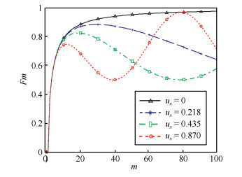
The curves of $F_m$ with different values of $u_x$ are shown in Fig. 4,in which $u_x=0$ with solid line,$u_x=0.218$ with the short dotted blue line,$u_x=0.435$ with dashed-dot green line,and $u_x=0.870$ with the short dotted red line,respectively. As can be seen from Fig. 4 that the behavior of the optimal fidelity $F_m$ is fluctuant and periodic,whose period depends on the value of $u_x$. The period decreases as the $u_x$ increases. The period which corresponds to the measurement number $N$ equals 40 when $u_x=0.870$,and the peak value of $F_m$ in the first period cannot reach performance of $95 \%$. However,the peak ${F_m}$ in the second period ($m = 79$) can reach $96.84 \%$. Especially,the peak value of $F_m$ increases as the number of period increases. Experiments show that the peak value of $F_m$ turns to be $99.68 \%$ with $m$ approaching 1000,which is much different from the results in the case with only one external control field used in Case 1 of Section Ⅲ-C,where the $F_m$ is a convex curve without periodicity. The simulation result indicates that the periodic peak value of $F_m$ can infinitely approach to 1 as long as the number of measurement is large enough.

|
Download:
|
| Fig. 4 The curve of optimal fidelity $F_m$ with different control field $u_x$ | |
By comparing and analyzing the results in Case 1 and Case 2,we
can conclude that the control field of $u_y$ is effective for the
reduction of measurement number to meet the performance. While the
control field of $u_x$ plus $u_z$ can reach the optimal fidelity
as high performance as possible,which is often used in the actual
experiments,for example in the manipulation of a double
quantum-dot charge qubit
This paper investigated the manipulation between eigenstates of a two-level quantum system by optimal measurements. The instantaneous projective measurements were used to drive the state from one eigenstate to another. The three cases manipulations were studied,and the analytical solutions were derived. Three kinds of numerical simulations of the manipulation were performed,in which characteristics of the optimal measurement-based control were analyzed,and the optimal parameters in different cases were obtained. The simulation experimental results verify the validity of the optimal measurement-based control,and indicate that the free evolution may affect the effectiveness of the manipulation, which can be compensated by the external control fields. Of course,the actual systems need to consider many other complex factors. The optimal measurement control and the external control fields proposed in this paper can be implemented by the open-loop control system. We believe that one can obtain better quantum state manipulation performance under advanced control methods and technologies.
| [1] | Huang G M, Tarn T J, Clark J W. On the controllability of quantummechanical systems. Journal of Mathematical Physics, 1983, 24(11):2608-2618 |
| [2] | Peirce A P, Dahleh M A, Rabitz H. Optimal control of quantummechanical systems:existence, numerical approximation, and applications. Physical Review A, 1988, 37(12):4950-4964 |
| [3] | Palao J P, Kosloff R. Quantum computing by an optimal control algorithm for unitary transformations. Physical Review Letters, 2002, 89(18):188301 |
| [4] | Montangero S, Calarco T, Fazio R. Robust optimal quantum gates for Josephson charge qubits. Physical Review Letters, 2007, 99(17):170501 |
| [5] | Maximov I I, Tošner Z, Nielsen N C. Optimal control design of NMR and dynamic nuclear polarization experiments using monotonically convergent algorithms. Journal of Chemical Physics, 2008, 128(18):184505 |
| [6] | Eitan R, Mundt M, Tannor D J. Optimal control with accelerated convergence:combining the Krotov and quasi-Newton methods. Physical Review A, 2011, 83(5):053426 |
| [7] | Shuang F, Rabitz H. Cooperating or fighting with control noise in the optimal manipulation of quantum dynamics. The Journal of Chemical Physics, 2004, 121(19):9270-9278 |
| [8] | Judson R S, Rabitz H. Teaching lasers to control molecules. Physical Review Letters, 1992, 68(10):1500-1503 |
| [9] | Mendes R V, Manko V I. Quantum control and the Strocchi map. Physical Review A, 2003, 67(5):053404 |
| [10] | Hwang B, Goan H S. Optimal control for non-Markovian open quantum systems. Physical Review A, 2012, 85(3):032321 |
| [11] | Pechen A, Ilin N, Shuang F, Rabitz H. Quantum control by von Neumann measurements. Physical Review A, 2006, 74:052102 |
| [12] | Shuang F, Rabitz H. Cooperating or fighting with decoherence in the optimal control of quantum dynamics. The Journal of Chemical Physics, 2006, 124(15):154105 |
| [13] | Shuang F, Rabitz H, Dykman M. Foundations for cooperating with control noise in the manipulation of quantum dynamics. Physical Review E, 2007, 75(2):021103 |
| [14] | Shuang F, Zhou M L, Pechen A, Wu R B, Shir O M, Rabitz H. Control of quantum dynamics by optimized measurements. Physical Review A, 2008, 78(6):063422 |
| [15] | Zhu W S, Rabitz H. Closed loop learning control to suppress the effects of quantum decoherence. The Journal of Chemical Physics, 2003, 118(15):6751-6757 |
| [16] | Roa L, Delgado A, Ladrón de Guevara M L, Klimov A B. Measurementdriven quantum evolution. Physical Review A, 2006, 73(1):012322 |
| [17] | Gong J B, Rice S A. Measurement-assisted coherent control. The Journal of Chemical Physical, 2004, 120(21):9984-9988 |
| [18] | Sugawara M. Quantum dynamics driven by continuous laser fields under measurements:towards measurement-assisted quantum dynamics control. The Journal of Chemical Physics, 2005, 123(20):204115 |
| [19] | Sugawara M. Measurement-assisted quantum dynamics control of 5-level system using intense CW-laser fields. Chemical Physics Letters, 2006, 428(4-6):457-460 |
| [20] | Yamamoto N, Hara S. Relation between fundamental estimation limit and stability in linear quantum systems with imperfect measurement. Physical Review A, 2007, 76(3):034102 |
| [21] | Shuang F, Pechen A, Ho T S, Rabitz H. Observation-assisted optimal control of quantum dynamics. The Journal of Chemical Physics, 2007, 126(13):134303 |
| [22] | Doherty A C, Jacobs K. Feedback control of quantum systems using continuous state estimation. Physical Review A, 1999, 60(4):2700-2711 |
| [23] | Vijay R, Macklin C, Slichter D H, Weber S J, Murch K W, Naik R, Korotkov A N, Siddiqi I. Stabilizing Rabi oscillations in a superconducting qubit using quantum feedback. Nature, 2012, 490(7418):77-80 |
| [24] | Brakhane S, Alt W, Kampschulte T, Martinez-Dorantes M, Reimann R, Yoon S, Widera A, Meschede D. Bayesian feedback control of a twoatom spin-state in an atom-cavity system. Physical Review Letters, 2012, 109(17):173601 |
| [25] | Wang Y X, Wu R B, Chen X, Ge Y J, Shi J H, Rabitz H, Shuang F. Quantum state transformation by optimal projective measurements. Journal of Mathematical Chemistry, 2011, 49(2):507-519 |
| [26] | Yan Y, Zou J, Xu B M, Li J G, Shao B. Measurement-based direct quantum feedback control in an open quantum system. Physical Review A, 2013, 88(3):032320 |
| [27] | Cong S, Gao M Y, Cao G, Guo G C, Guo G P. Ultrafast manipulation of a double quantum-dot charge qubit using Lyapunov-based control method. IEEE Journal of Quantum Electronics, 2015, 51(8):8100108 |