RECENTLY,a variety of mechanical systems have received significant attention in research communities ^{[1,2,3,4,5,67]}. However,in the field of control practices,various kinds of severe uncertainties cannot help but accompany mechanical systems^[8]. Among these uncertainties,a situation where control designers cannot access the actual actuator dynamics is considered as an obstacle to achieve the satisfying performance. Hence,the high quality performance or even the control stability is ineluctably challenged in presence of unknown actuator nonlinearities.

The promising solution to the unknown control coefficients problem was reported in ^[9],where a Nussbaum gain based method was originally proposed for first-order linear systems. Subsequently,adaptive control approaches associated with Nussbaum gains were proposed in ^[10]. Remarkable progresses were achieved in ^{[11, 12, 13]} for a single input single output (SISO) system. Moreover,Yang et al.^{[14, 15]} creatively developed a discrete Nussbaum gain based output feedback control to handle nonlinear systems with unknown control gains. Liu^[16] further investigated output-feedback adaptive stabilization for nonlinear systems with unknown control coefficients,where the limitation of the priori knowledge about control gain sign is removed. With the combination of Nussbaum gain with adaptive backstepping algorithm,Du et al.^[17] creatively proposed a novel adaptive robust autopilot for ships in the presence of both parameter uncertainties and disturbances with unknown bound. Moreover,an exciting result was further obtained in ^[18] by extending to an uncertain ship model with unknown time-variant parameters. Most recently, Du et al.^[19] developed a promising control scheme for the course control problem of ships with parameter uncertainties and unknown control coefficients by utilizing the dynamic surface control and the Nussbaum gain. Hu^[20] successfully realized attitude tracking and vibration stabilization of a flexible spacecraft,where the Nussbaum gain technique and adaptive mechanisms are employed to relax the sign assumption. In these SISO systems,only one Nussbaum gain is required to investigate one unknown coefficient^[21]. However,both the control design and analysis become more difficult when each subsystem needs one Nussbaum gain in multiple input multiple output (MIMO) systems.

In fact,such difficulty implies that it is not ensured in theory to extend the Nussbaum gain from one to multiple. To realize the extension,some pioneering works ^{[22, 23, 24, 25, 26, 27]} have been conducted to handle each subsystem’s control coefficient by utilizing the decentralized based approaches. Boulkroune et al.^[28] successfully proposed an adaptive fuzzy control method to deal with unknown sign of the control gain for a class of MIMO nonlinear systems. Furthermore,Arefi et al.^[29] artfully investigated uncertain MIMO nonlinear systems with unavailable system states and an unknown sign of control gain matrix. Chen et al.^[30] performed an outstanding research to solve the difficulty from the coexistence of multiple Nussbaum gains. Furthermore,progress has been achieved in ^[31] to extend the Nussbaum tool^[30] from constant coefficients to time-varying ones. Moreover,Ding^[32] successfully took a further step forward to remove the limitation of the prior knowledge of constant coefficients’ upper and lower bounds, and creatively constructed a promising scheme to realize the output control of multi-agent system.

Though remarkable progresses have been achieved,existing literatures work are based on the assumption that unknown control coefficients should be constant or the upper and lower bounds of control coefficients should be available as the prior knowledge. However,for many mechanical systems,the actuator dynamics (the control coefficient) not only is unknown to the control procedure,but also performs nonlinearly. Particularly, nonlinearities and uncertainties including backlash, saturation,hysteresis,and deadzone are common phenomena in many systems ^{[8, 33, 34, 35, 36, 37, 38, 39, 40, 41, 42, 43]}. Due to the nonsmooth time-varying characteristic,these nonlinearities may result in the control failure or the instability^[8]. Hence,it is a meaningful but challenging task to elucidate whether there exists a solution to control MIMO mechanical systems involving unknown timevarying actuator nonlinearities without any prior knowledge of unknown actuators.

Motivated by above analyses,an adaptive control scheme is developed for MIMO mechanical systems with unknown actuator nonlinearities. The main properties of this paper are presented as follows:

1) A powerful Nussbaum analysis tool is presented in Theorem 1,where the control problem from unknown time-varying input coefficients and their signs are simultaneously tackled without any prior knowledge of input coefficients. Therefore,it lays the groundwork for realizing MIMO mechanical systems with unknown actuator nonlinearities.

2) As shown in Theorem 2,the developed Nussbaum analysis tool is successfully combined with adaptive robust control. Hence,unknown bounded disturbances from timevarying actuator nonlinearities are compensated in the stability analysis. Moreover,the proposed control is not limited to mechanical systems and can be applied to large-scale nonlinear systems.

The mechanical system can be expressed as the following dynamical process^{[1, 8,44,45]}:

where $r\in R^{L\times 1}$ denotes the displacement; $\dot r\in R^{L\times 1}$ denotes the velocity; $W(r)\in {\bf R}^{L\times L}$ is the inertial matrix; $H (r ,{\dot r} )\in {\bf R}^{L\times L}$ denotes the Coriolis and centrifugal matrix; $G(r)\in R^{L\times 1}$ denotes the gravitational force vector; and $u\in R^{L\times 1} $ denotes the actual torque or force being exerting on the mechanical system. It is noted that the torque or force $u$ is affected by unknown actuator nonlinearities. Therefore,$u$ can be described mathematically
as ^{[33, 35, 38, 39, 40, 41, 42, 46, 47]}

where $\tau$ is the control law to be designed; the time-varying matrix $\vartheta(t)\in R^{L\times L}$ is given as $\vartheta(t)={\rm diag}[{\vartheta}_1(t),... , {\vartheta}_i(t),... ,{\vartheta}_L(t)]$; and ${T}\in {\bf R}^{L\times 1} $ is the unmodelled vector. It is noted that ${\vartheta}_i(t)$ is bounded for $i=1,... ,L$,but its upper or lower bounds are unknown. Each element of the vector ${T}$ in (2) satisfies $\vert {T_i}\vert\le K_{r_{i}}$ with $K_{r_{i}}$ being an unknown constant.

Remark 1. The practical significance of (2) stems from the existence of unknown actuator nonlinearities. As shown in remarkable works ^{[33, 35, 38, 39, 40, 41, 42, 46, 47]},(2) is not limited to describe a certain kind of the actuator nonlinearity,but has the capacity of modelling actuator nonlinearities including hysteresis,deadzone,and saturation in many physical applications. As a result,(2) denotes a unified mathematical form,which is suitable to model a wide range of actuator nonlinearities.

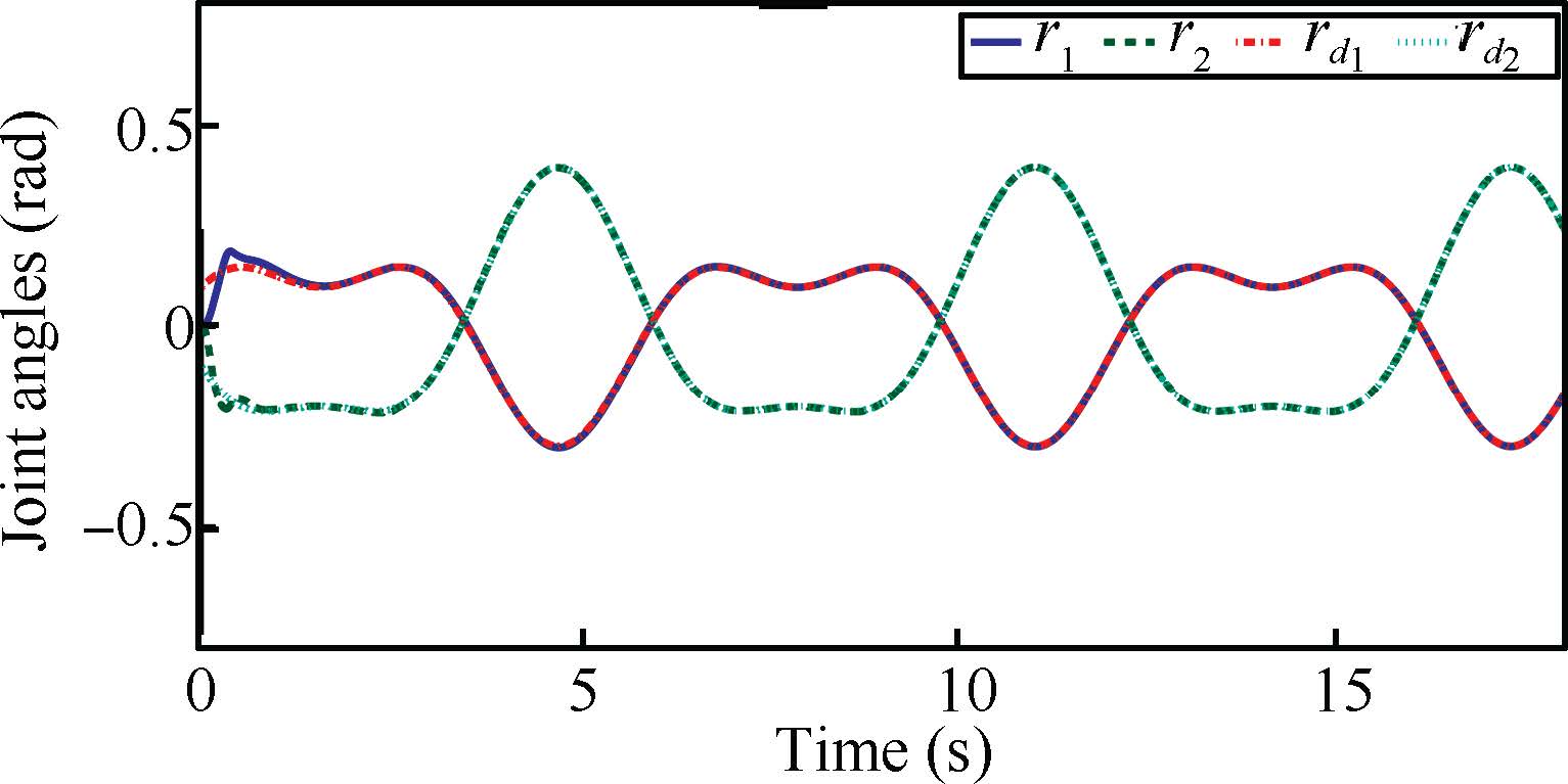
The control objective is to establish a novel Nussbaum analysis tool for MIMO systems and to design an appropriate and effective control input $\tau$ for the mechanical system with unknown actuator nonlinearities. After applying the control law $\tau$, one obtains that the displacement and the velocity should converge to the desired trajectories,respectively. That is, $r(t)\rightarrow r_d(t)$ and $\dot r(t)\rightarrow \dot r_d(t)$, where $(\cdot)_d$ means the desired trajectory.

To facilitate the control analysis,three properties are summarized as follows ^[1,8,44,45]:

Property 1. The matrix $W(r) $ is symmetric positive definite.

Property 2. The matrix $\big\{2H (r,\dot r )-\dot W (r )\big\}$ is skew-symmetric.

Property 3. Three terms at the left hand of (1) can be reformulated as $ {W} (r ){\ddot r_e } +{H} (r ,{\dot r } ){ \dot r_e} +{G} (r )=\Theta(r,\dot r,\dot r_e,\ddot r_e)\aleph,$ where the constant vector $\aleph$ denotes physical parameters of the mechanical system; $\dot r_e$ $R^{L\times 1}$ is defined as the reference velocity error with $ \dot r_e=\dot r_d-\delta\tilde{r}$,$\tilde{r}=r-r_d$ and $\delta\in{\bf R}^{L\times L}$ being a symmetric positive definite matrix; $\ddot r_e$ denotes the time derivative of $ \dot r_e$; and $\Theta(r, \dot r,\dot r_e,\ddot r_e)$ is defined as the regression matrix.

A Nussbaum gain based control approach is usually used to investigate unknown control coefficients. The main question is how to remove the limitation of prior knowledge of time-varying coefficients' upper and lower bounds. To get rid of the dilemma,a novel Nussbaum gain is modified from ^[32]:

where $\hbar$ denotes a real variable.

Proposition 1. Derived from the observation of the proposed definition (3),four important properties of $\mathcal{G}_N(\hbar)$ are presented as:

1) $\mathcal{G}_N(\hbar)$ is an odd function with $\hbar$ being a real variable. Moreover,the integration of $\mathcal{G}_N(\hbar)$ over the interval $[0,\hbar]$ is defined as $\mathcal{G}_T(\hbar)=\int_0^\hbar\mathcal{G}_N(\chi){\rm d}\chi$. Hence,$\mathcal{G}_T(\hbar)$ is even with respect to $\hbar$.

2) The minimal value of $\mathcal{G}_T(\hbar)$ over the interval $\hbar\in[0,2k\pi+\pi]$ can be derived at $\hbar=2k\pi+\pi$ and its minimum can be calculated as $\mathcal{G}_{T_{\rm min}}=-\exp\left({\frac{(2k\pi+\pi)^2}{2}}\right)-1$,where $k$ is a positive integer. The maximal value of $\mathcal{G}_T(\hbar)$ over the interval $ \hbar\in[0,2k\pi+\pi]$ can be obtained at $\hbar=2k\pi$ and its maximum can be computed as $\mathcal{G}_{T_{\rm max}}=\exp\left({\frac{(2k\pi)^2}{2}}\right)-1$.

3) As $\hbar$ approaches the infinity,$\mathcal{G}_N(\hbar)$ is one choice of Nussbaum-type gains^[9],which satisfy following two constraints mathematically: $\lim\nolimits_{\hbar\rightarrow+\infty}{\sup\left\{\int_0^\hbar{\mathcal{G}_N(\chi){\rm d}\chi}\right\}}=+\infty$; and $\lim\nolimits_{\hbar\rightarrow+\infty}{\inf\left\{\int_0^\hbar{\mathcal{G}_N(\chi){\rm d}\chi}\right\}}=-\infty$.

4) The proposed function $\mathcal{G}_N(\hbar)$ belongs to one choice of Ryan-type Nussbaum gains^[48] such that the following properties hold: $\lim_{\hbar\rightarrow+\infty}{\sup\left\{\frac{1}{\hbar}\int_0^\hbar{\mathcal{G}_N(\chi){\rm d}\chi}\right\}}=+\infty$; and $\lim_{\hbar\rightarrow+\infty}{\inf\left\{\frac{1}{\hbar}\int_0^\hbar{\mathcal{G}_N(\chi){\rm d}\chi}\right\}}=-\infty. $

Proof.

1) From the definition of (3),we obtain that

Therefore,it is derived that the proposed Nussbaum gain is an odd function. As an immediate result,its integration is an even function.

2) Utilizing the integration theorem and the definition (3),we can derive that

Hence,the minimal and maximal values of $\mathcal{G}_T(\hbar)$ over the interval $\hbar\in[0,2k\pi+\pi]$ are derived at $\hbar=2k\pi+\pi$ and $\hbar=2k\pi$,respectively. Immediately,its minimum and maximum can be computed as $\mathcal{G}_{T_{\rm min}}=\mathcal{G}_T(2k\pi+\pi)=-\exp\left({\frac{(2k\pi+\pi)^2}{2}}\right)-1$ and $\mathcal{G}_{T_{\rm max}}=\mathcal{G}_T(2k\pi)=\exp\left({\frac{(2k\pi)^2}{2}}\right)-1$, respectively.

3) From the result in Proposition 1-2),the minimal and maximum values of $\mathcal{G}_T(\hbar) $ over the interval $[2k\pi$, $2k\pi+\pi]$ can be obtained at $\hbar=2k\pi+\pi$ and $\hbar=2k\pi$, respectively. Hence,Proposition 1.3) can be proved if following two relations are satisfied: $\lim\nolimits_{k\rightarrow+\infty}{\sup\int_0^{2k\pi}{\mathcal{G}_N(\chi){\rm d}\chi}}=+\infty$; and $\lim\nolimits_{k\rightarrow+\infty}{\inf\int_0^{2k\pi+\pi}{\mathcal{G}_N(\chi){\rm d}\chi}}=-\infty$. To prove the former,the integration $\int_0^{2k\pi}{\mathcal{G}_N(\chi){\rm d}\chi}$ can be computed directly from (5) as $\int_0^{2k\pi}{\mathcal{G}_N(\chi){\rm d}\chi}=\exp\left({\frac{(2k\pi)^2}{2}}\right)-1$. As $k$ approaches infinity,it yields $\lim_{k\rightarrow+\infty}{\sup\left\{\int_0^{2k\pi}{\mathcal{G}_N(\chi){\rm d}\chi}\right\}}=+\infty$. Similarly,we have $\lim_{k\rightarrow+\infty}{\inf\left\{\int_0^{2k\pi+\pi}{\mathcal{G}_N(\chi){\rm d}\chi}\right\}}=-\infty$.

4) There exists an increasing sequence $\{\hbar_k\}$ satisfying $\hbar_k=2k\pi$,where $\hbar_k$ approaches infinity as $k$ approaches infinity. Therefore,the following inequality holds ${\sup\left\{\frac{1}{\hbar}\int_0^\hbar{\mathcal{G}_N(\chi){\rm d}\chi}\right\}} \geq {{\frac{1}{\hbar_k}\int_0^{\hbar_k}{\mathcal{G}_N(\chi){\rm d}\chi}}}$. As proofed in Proposition 1.1)-3), ${\int_0^{2k\pi}{\mathcal{G}_N(\chi){\rm d}\chi}}=\mathcal{G}_T(2k\pi)=\exp\left({\frac{(2k\pi)^2}{2}}\right)-1$. As $k$ increases,the term $ \exp\left({\frac{(2k\pi)^2}{2}}\right)-1$ increases faster than the term $2k\pi$ does. Moreover,as $k $ approaches infinity,it yields $\lim_{k\rightarrow+\infty}{\left\{\frac{\exp\left({\frac{(2k\pi)^2}{2}}\right)-1}{2k\pi}\right\}}=+\infty$. Therefore,it yields that $\lim_{\hbar\rightarrow+\infty}{\sup\left\{\frac{1}{\hbar}\int_0^\hbar{\mathcal{G}_N(\chi){\rm d}\chi}\right\}}=+\infty$. As a similar result of above equation,we have an increasing sequence $\{\hbar_k'\}$ which satisfies $\hbar_k'=2k\pi+\pi$,where $\hbar_k'$ approaches infinity as $k$ approaches infinity. The following inequality holds ${\inf\left\{\frac{1}{\hbar}\int_0^\hbar{\mathcal{G}_N(\chi){\rm d}\chi}\right\}}\leq {\left\{\frac{\int_0^{2k\pi+\pi}{\mathcal{G}_N(\chi){\rm d}\chi}}{2k\pi+\pi}\right\}}$. Since $\lim_{k\rightarrow+\infty}{\left\{\frac{-\exp\left({\frac{(2k\pi+\pi)^2}{2}}\right)-1}{2k\pi+\pi}\right\}}=-\infty$, we obtain that $ \lim_{\hbar\rightarrow+\infty}{\inf\left\{\frac{1}{\hbar}\int_0^\hbar{\mathcal{G}_N(\chi){\rm d}\chi}\right\}}=-\infty. $

Having seen $\mathcal{G}_N(\hbar)$'s important properties in Proposition 1,we will not only tackle the control problem from multiple Nussbaum gains coexisting in one Lyapunov function candidate,but also remove the limitation of the prior knowledge of varying parameters' upper and lower bounds. The main result is summarized as Theorem 1.

Theorem 1. Suppose that the time-varying function ${\vartheta}_i(t)$ is defined in an unknown closed interval $\nabla=[{\vartheta}^{-},{\vartheta}^{+}]$ with $0\notin \nabla$, ${\vartheta}^{-}:= \min\nolimits_{1\leq i\leq L}\{{\vartheta}_{i}(t)\}$ and ${\vartheta}^{+}:=\max\nolimits_{1\leq i\leq L}\{{\vartheta}_{i}(t)\}$. Let $V(t,x(t))$ be a smooth positive definite function defined on the time interval $[0,t_f)$. $\hbar_i(t)$ is designed as a smooth function with $\hbar_i(0)$ being bounded for $i=1,2,... ,n$. Define $\eta_i$ and $\varpi$ to be known constants. If the following inequality holds:

then the conclusion is drawn that $\hbar_i(t)$, $V(t,x(t))$ and ${{\vartheta}_i(t)\mathcal{G}_N(\hbar_i(t))\dot \hbar_i(t)}$ must be bounded on $[0,t_f)$ for $i=1,... ,L$.

Proof.

Now that the above inequality holds over the time interval $[0, t_f)$,it is thus derived that the following constraint holds

where the bounded variable $\varpi_1$ is defined as $\varpi_1=\sum_{i=1}^{L}\int_{\hbar_i(0)}^0{{\vartheta}_i(\chi) \mathcal{G}_N(\chi){\rm d}\chi}-\sum_{i=1}^{L}{\eta_i\hbar_i(0)}+\varpi$. The remaining proof is accomplished by seeking a contradiction. In what follows, some $\hbar_i(t)$ are supposed to be bounded,but some are unbounded over $[0,t_f)$ for $i=1,... ,L$. Hence,we have $\hbar_1(t), ... ,\hbar_\xi(t) $ are unbounded for $1\leq \xi \leq L$, meanwhile $\hbar_{\xi+1}(t),... ,\hbar_L(t)$ remain bounded. Considering each actuator has an unknown identical control direction,the contradiction is,therefore,carried out into following two cases.

Case 1. Each actuator has a positive control sign.

$\{t_k\}$ is defined as $t_k = \min\{t:|\hbar_i(t)|=2k\pi+\pi\ |\ {1\leq i\leq \xi}\}$.

When $k\rightarrow\infty$,it is obtained that $t_k \rightarrow t_f$. The reason is presented as follows. The smooth function $\hbar_i(t)$ is assumed to be unbounded on $[0,t_f)$ for $1\leq i\leq \xi$. When $k\rightarrow\infty$,it is obtained that $\hbar_i(t)=2k\pi+\pi$ must approach the infinity (or $\hbar_i(t)=2k\pi+\pi$ must be unbounded). Therefore,$t$ is approaching $t_f$ if $\hbar_i(t)$ is unbounded. Moreover, recalling the definition of $t_k$,we have $t_k\rightarrow t_f $ as $t\rightarrow t_f$. As a result,the conclusion is obtained that when $k\rightarrow\infty$,it is obtained that $t_k\rightarrow t_f$. A similar result has been obtained in ^[30]. Moreover, within the frame of $t_k'$s definition,one has $|\hbar_{i'_k}(t_k)|=2k\pi+\pi$ for $1\leq i'_k \leq \xi$. When faced with the condition that $i $ is not equal to $i'_k$,we have $|\hbar_i(t)|\leq2k\pi+\pi$. Combining the results in (6) and (5), $V(t,x(t))$ at the specified time $t=t_k$ can be rewritten as

Utilizing results in Proposition 1,one obtains that the maximum value of $\mathcal{G}_T(\hbar_i(k))$ over $\hbar_i(k)\in[0,2k\pi+\pi] $ is obtained at $\hbar_i(k)=2k\pi$. Moreover,$\mathcal{G}_N(\hbar_i(k))$ must be non-negative over $\hbar_i(k)\in[2k\pi-\pi,\ 2k\pi]$. As a result of this property, $\sum_{\{i=1,i\neq i'_k\}}^{l}\int_0^{\hbar_i(t)}{ {\vartheta}_i(\chi)\mathcal{G}_N(\chi){\rm d}\chi}$ in (7) can be further reformulated as:

where $\bar{\vartheta}_{\xi}={\vartheta}_{max}(\xi-1)$. Considering the fact that $|\hbar_{i'_k}(t_k)|=2k\pi+\pi$,$1\leq i'_k \leq \xi$,it is thus derived that the remaining analyses should be decomposed into two subcases. That is, $\hbar_{i'_k}(t_k)=2k\pi+\pi$ and $\hbar_{i'_k}(t_k)=-2k\pi-\pi$.

Subcase 1. $\hbar_{i'_k}(t_k)=2k\pi+\pi$. Consequently,the term $\int_0^{\hbar_{i'_k}(t_k)}{ {\vartheta}_{i'_k}(\chi)\mathcal{G}_N(\chi){\rm d}\chi}$ at right hand of (7) is changed into

As an immediate result of Proposition 1,it is obtained that $\mathcal{G}_N(\hbar_i(k))\leq0$ holds when $\hbar_i(k)$ belongs to the interval $[{2k\pi},{2k\pi+\pi}]$. Therefore, $\int_0^{\hbar_{i'_k}(t)}{ {\vartheta}_{i'_k}(\chi)\mathcal{G}_N(\chi){\rm d}\chi}$ in (9) can be rewritten as

Based on results in (8) -- (10),(7) can be reformulated as

where $\varpi_2=\sum_{i=\xi+1}^{L}\int_0^{\hbar_i(t_k)}{ {\vartheta}_i(\chi)\mathcal{G}_N(\chi){\rm d}\chi}+\varpi_1+\sum_{i=\xi+1}^{L}{\eta_i\hbar_i(t_k)}$. When $i$ is chosen as $\xi+1\leq i\leq L$,both $\int_0^{\hbar_i(t_k)}{ {\vartheta}_i(\chi)\mathcal{G}_N(\chi){\rm d}\chi}$ and $\hbar_i(t_k)$ are bounded. Hence,it is obtained that $\sum_{i=\xi+1}^{L}\int_0^{\hbar_i(t_k)}{ {\vartheta}_i(\chi)\mathcal{G}_N(\chi){\rm d}\chi}$ and $\sum_{i=\xi+1}^{L}{\eta_i\hbar_i(t_k)}$ must be bounded. As an immediate result,$\varpi_2$ is also bounded. After applying the definition of $\mathcal{G}_T(\hbar)$ in (5),one can change (11) into

Employing the definition of $t_k$,one obtains that $|\hbar_i(t_k)|\leq 2k\pi+\pi$ holds for $1\leq i\leq \xi$. Subsequently,the following constraint must hold $\sum_{i=1}^{\xi}{\eta_i\hbar_i(t)}\leq 2\bar\eta {\xi}k\pi+\bar\eta\xi\pi$,where $\bar\eta$ denotes the maximum value of $|\eta_i|$ for $1\leq i\leq \xi$. $\big\{\xi{\vartheta}_{\rm max} \mathcal{G}_T(2k\pi)+{\vartheta}_{\rm min} \mathcal{G}_T(2k\pi+\pi)+\sum_{i=1}^{\xi}{\eta_i\hbar_i(t)}\big\}$ in (12) is rewritten as

where the definition of $\mathcal{G}_T(\hbar)$ in (5) is employed. Moreover,as $\exp\left({\frac{\pi(4k\pi+\pi)}{2}}\right)$ in (13) will dominate any bounded functions with a sufficiently large $k$, the sign of $\Big\{{{\vartheta}_{\rm min}}\exp\left({\frac{\pi(4k\pi+\pi)}{2}}\right)-\xi{\vartheta}_{\rm max}\Big\}$ is thus negative as $k$ approaches $\infty$. Therefore,the following constraint must hold

when $k $ approaches infinity. Similarly,the first two terms at the right hand of (12) also satisfy

Similar to (14),(15) is thus changed into

where $k \rightarrow \infty$.

Combining results in (14) and (16),one obtains that the following property holds

where $k \rightarrow \infty$. Moreover, $\sum_{i=1}^{\xi}\int_0^{2k\pi-\pi}{ {\vartheta}_i(\chi)\mathcal{G}_N(\chi){\rm d}\chi}$ at the right hand of (12) can be reformulated as

Considering the fact that $\mathcal{G}_N(\chi) < 0$ over the interval (0,$\pi$) and $\mathcal{G}_N(0)=0$,it is thus derived that $\int_0^{\pi}{ {\vartheta}_i(\chi)\mathcal{G}_N(\chi){\rm d}\chi} < 0$. From observation of (18),each new element $\sum_{i=1}^{\xi}\int_{2k\pi-3\pi}^{2k\pi-\pi}{ {\vartheta}_i(\chi)\mathcal{G}_N(\chi){\rm d}\chi}$ is thus added to $\sum_{i=1}^{\xi}\int_0^{2k\pi-\pi}{ {\vartheta}_i(\chi)\mathcal{G}_N(\chi){\rm d}\chi}$ as the positive integer $k$ increases. Therefore,the sign of $\sum_{i=1}^{\xi}\int_0^{2k\pi-\pi}{ {\vartheta}_i(\chi)\mathcal{G}_N(\chi){\rm d}\chi}$ can be determined if the sign of $\sum_{i=1}^{\xi}\int_{2k\pi-3\pi}^{2k\pi-\pi}{ {\vartheta}_i(\chi)\mathcal{G}_N(\chi){\rm d}\chi}$ is determined. By decomposing the interval [$2k\pi-3\pi$,$2k\pi-\pi$] into [$2k\pi-3\pi$,$2k\pi-2\pi$] $\bigcup$ [$2k\pi-2\pi$, $2k\pi-\pi$],one obtains that $\sum_{i=1}^{\xi}\int_{2k\pi-3\pi}^{2k\pi-\pi}{ {\vartheta}_i(\chi)\mathcal{G}_N(\chi){\rm d}\chi}$ is changed into

Employing similar analysis as in (13)-(17),one can conclude that when $k$ approaches $\infty$,the newly added element $\sum_{i=1}^{\xi}\int_{2k\pi-3\pi}^{2k\pi-\pi}{ {\vartheta}_i(\chi)\mathcal{G}_N(\chi){\rm d}\chi}$ approaches $-\infty$. Subsequently,it is derived that the following constraint must hold

At this stage,$V(t_k,x(t_k))$ can be further rewritten as follows by combining results in (12)-(19):

From the observation of (20),it is easy to obtain that a contradiction is generated. Therefore,all of $\hbar_i(t)$ for $1\leq i\leq L$ is bounded over $[0,t_f)$. Thus,$V(t,x(t))$ and $\sum_{i=1}^{L}\int_0^t{{\vartheta}_i(t)\mathcal{G}_N(\hbar_i(t))\dot \hbar_i(t) {\rm d} t}$ are also bounded over $[0,t_f)$.

Subcase 2. $\hbar_{i'_k}(t_k)=-2k\pi$. It is noted that the investigated Nussbaum gain is defined as an odd function (see Proposition 1). Therefore, the proof of Subcase 2 can be easily obtained based on the procedure of Subcase 1. Hence,Subcase 2 is omitted here.

Case 2. Each actuator has a negative sign.

Here,$\{t_k\}$ is redefined as $ t_k = \min\{t:|\hbar_i(t)|=2k\pi+2\pi\ | \ {1\leq i\leq \xi}\}, $ where $t_k \rightarrow t_f$ as $k\rightarrow\infty$. Using the similar technique developed in Case 1,one obtains that the remaining proof of Case 2 can be derived.

Employing the control design in ^[8],one defines the filtered tracking error as ${E}=\dot r- \dot r_e$. With the above definition,the control law $\tau$ is developed as:

where the vector $\hbar(t)$ is defined as $\hbar(t)=[\hbar_1(t),... ,\hbar_L(t)]^{\rm T}$; Nussbaum gain matrix $\overline{\mathcal{G}}_N(\hbar(t))$ is defined as $\overline{\mathcal{G}}_N(\hbar(t))={\rm diag}[\mathcal{G}_N(\hbar_1(t)),... , \mathcal{G}_N(\hbar_L(t))]$; and $ \bar \tau$ denotes a virtual controller. In particular,the virtual controller is given as

where $\hat\aleph$ is the estimate of $\aleph$; $\varphi$ is a positive definite matrix; Hyperbolic tangent function $\mbox{Tanh}({E}/{s_t})$ is designed as $\mbox{Tanh}({E}/{s_t})={\rm diag}[\tanh({s_1}/{s_t}),... ,\tanh({s_L}/{s_t})]$ with $s_t={1}/{(1+t^2)}$; and $\hat K_r $ is the estimate of $K_r$. $ \hbar(t)$ in $\mathcal{G}_N(\hbar(t))$ is updated by:

where the positive definite diagonal matrix ${\rm diag}(\beta)$ is designed as ${\rm diag}(\beta)={\rm diag}(\beta_{1},... ,\beta_{L})$; and the matrix ${\rm diag}(E) $ is defined as ${\rm diag}(E)={\rm diag}[E_1,... ,E_L]$. The adaptive parameters $\hat\aleph$ and ${\hat K}_r$ in the virtual controller (22) are updated by

where the matrix $\Psi$ is positive definite; and $\Theta(r,\dot r,\dot r_e,\ddot r_e)$ is the regression matrix.

Theorem 2. Given the mechanical system (1),the controller (21) and adaptive laws (23) - (25) ensure the asymptotic convergence of the system output.

Proof.

Construct a Lyapunov candidate as

where $\tilde{\aleph}=\hat\aleph-\aleph$. Taking the time derivation of (26),one has

Substituting the system dynamics (1) into (27),we have:

where the fact that $\big\{2H (r,\dot r )-\dot W (r )\big\}$ is skew-symmetric is employed (see Property 2). From (21) and (28), we have:

As an immediate result of (29),we obtain that

where $|E|^{\rm T}K_r -E^{\rm T} K_r\mbox{Tanh}({E}/{s_t}) < \sum_{i=1}^L0.2785s_tK_{r_i}$ is utilized. Substituting (23)-(25) into (30) leads to

Taking the integration of (31) over the interval [$0$,$t$] leads to

where $\varpi_a$ and $\varpi_b=\sum_{i=1}^L\int_0^t0.2785s_tK_{r_i}{\rm d}t+\varpi_a$ are bounded.

After applying Theorem 1 to (32),we have that $\hbar_i(t)$, $\int_0^t{{\vartheta}_i(t)\mathcal{G}_N(\hbar_i(t))\dot \hbar_i(t) {\rm d} t}$ and $V(t,x(t))$ are bounded over the time interval $[0, t_f)$ for $i=1,2,... ,L$. Hence,one has $t_f\rightarrow\infty$^[30]. From (32),$E^{\rm T}\varphi E$ must be integrable over $[0,\infty)$. Furthermore, $\lim\limits_{t\rightarrow\infty}E\rightarrow 0$ when Barbalat's Lemma is employed. It is derived that $r(t)\rightarrow r_d(t)$ and $\dot r(t)\rightarrow \dot r_d(t)$ as $t\rightarrow\infty$.

In what follows,a class of robotic arms are employed to testify the effectiveness of the proposed method. The dynamics is described as ^[8]

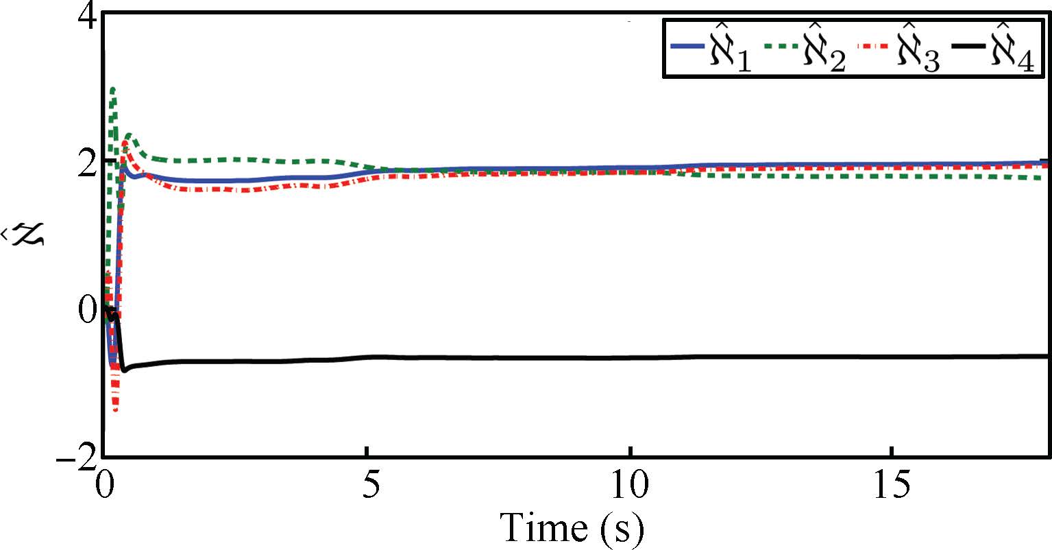
where $W_{11}=\aleph_1+2\aleph_3\cos(r_2)$; $W_{12}=W_{21}=\aleph_2+\aleph_3\cos(r_2)+\aleph_4\sin(r_2)$; $W_{22}=\aleph_2$; $H_{11}=-h\dot r_2$; $H_{12}=-h(\dot r_1+\dot r_2)$; $H_{21}=h\dot r_1$; $H_{22}=0$ and $h=\aleph_3\sin(r_2)-\aleph_4\cos(r_2)$ with $\aleph_1= 3.3$, $\aleph_2=0.97$,$\aleph_3=1.04$ and $\aleph_4=0.6$. Actuators nonlinearities are simulated as

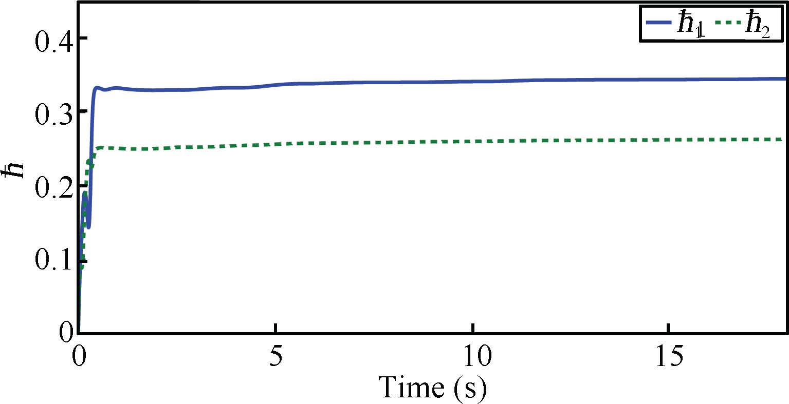
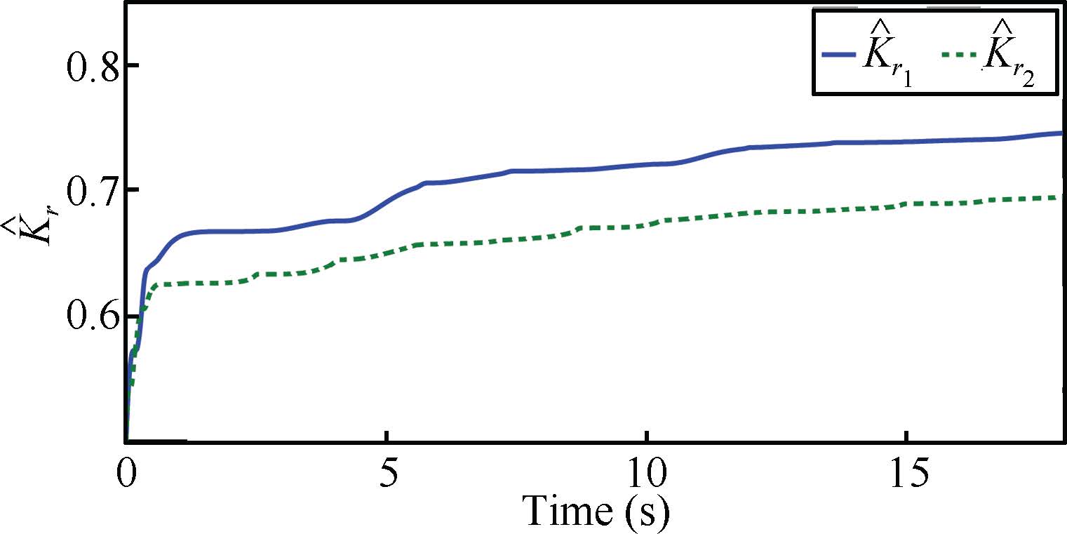
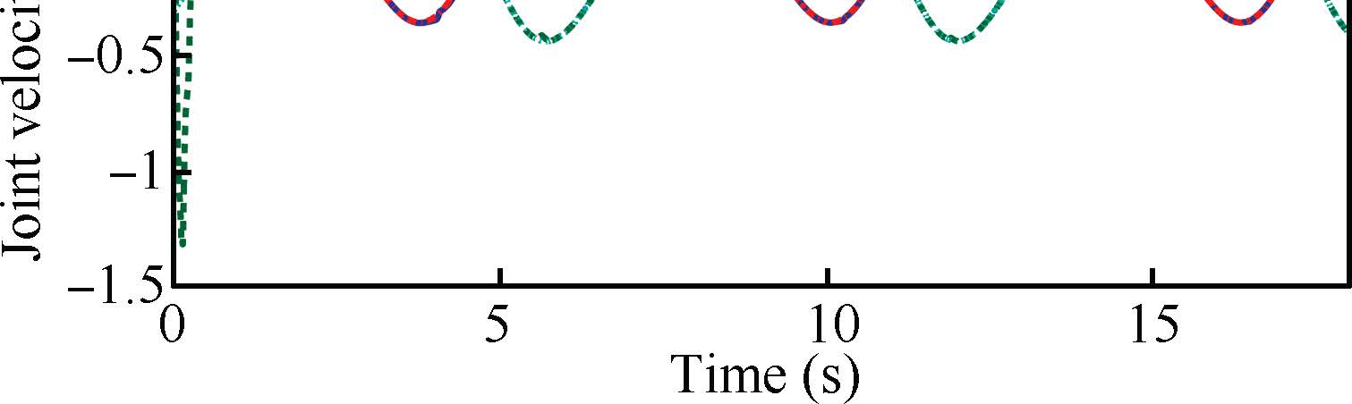
The desired trajectories are given as $ {r_d}(t) = [0.2\sin (t)+0.1\cos (2t),-0.3\sin(t)-0.1\cos(2t)]^{\rm T} {\rm rad}$ and ${\dot r_d}(t) = [0.2\cos (t)-0.2\sin (2t), -0.3\sin(t)+0.2\sin(2t)]^{\rm T} {\rm rad/s.} $ The initial joint angles and velocities are set as $r(0)=[0,0]^{\rm T} {\rm rad}$ and $\dot r(0)=[0,0]^{\rm T} {\rm rad/s}$, respectively. The initial value of $\hat\aleph(t)$ is designed as $\hat\aleph(0)=[0,0]^{\rm T}$. The updating gains $\hbar(t)$ and $K_r(t)$ are set initially as $\hbar(0)=[0,0]^{\rm T}$ and $K_r={\rm diag}[0.5,0.5]$. Gains are designed as $\varphi={\rm diag}[14,14]$,$\Psi={\rm diag}[10,10]$,$\delta={\rm diag}[10,10]$,and ${\rm diag}(\beta)={\rm diag}[0.1,0.1]$.

The simulation results are presented in Figs. 1-7. From the observation of Figs. 1-3,adaptive parameters including $\hbar$, $\hat\aleph$ and $\hat K_r$ are kept bounded after applying the proposed control. The performances of the mechanical system are carried out in Figs. 4 and 5,where joint angles and velocities quickly converge to the desired trajectories,respectively. Moreover,filtered tracking errors are plotted in Fig.6,where the asymptotic tracking is confirmed. The designed tracking control law is presented in Fig.7,where the boundedness is guaranteed after applying the proposed control.

Fig. 1

	Download: JPG larger image
Fig. 1. Adaptive parameters: $\hbar $.

Fig. 2

	Download: JPG larger image
Fig. 2. Adaptive parameters: ${\tilde \aleph }$.

Fig. 3

	Download: JPG larger image
Fig. 3. Adaptive parameters: ${{{\hat K}_r}}$.

Fig. 4

	Download: JPG larger image
Fig. 4. Joint angles.

Fig. 5

	Download: JPG larger image
Fig. 5. Joint velocities.

Fig. 6

	Download: JPG larger image
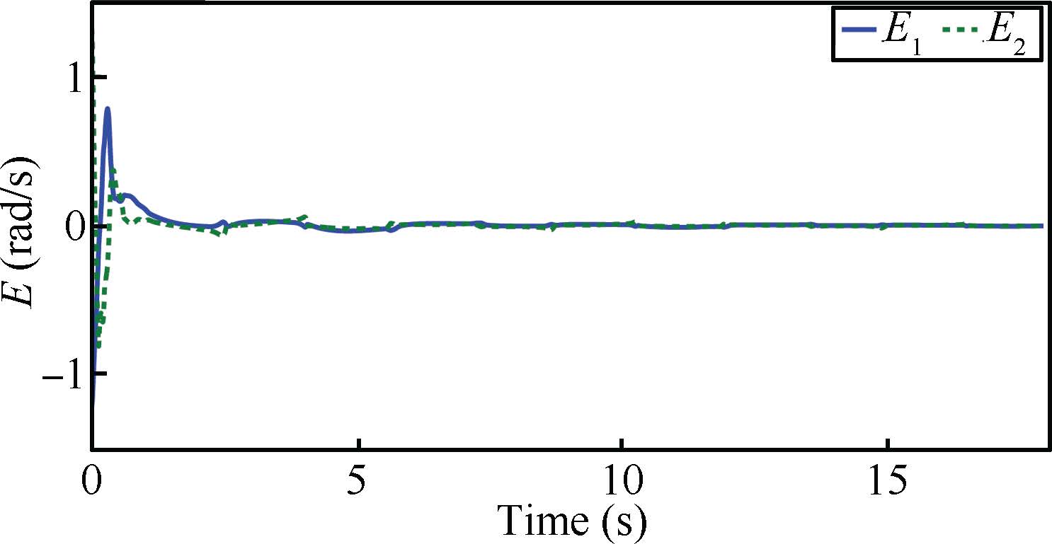
Fig. 6. Filtered tracking errors.

Fig. 7

	Download: JPG larger image
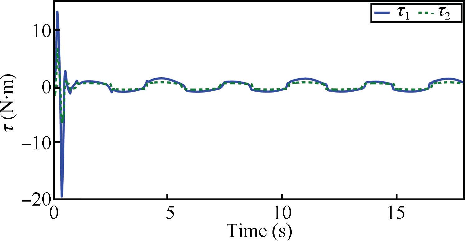
Fig. 7. The designed control law.

This paper has proposed an adaptive method for MIMO mechanical systems with unknown time-varying actuator nonlinearities. A new Nussbaum analysis tool is developed such that the requirement of the prior knowledge of time-varying nonlinearities is successfully removed. It has been theoretically proved that the proposed controller guarantees mechanical systems asymptotically converge to the desired trajectories in the sense of Lyapunov. A simulation example is performed to verify the effectiveness of the proposed approach.