M ICROGRID is a complicated cyber physical energy system (CPES) integrating a physical network including distributed energy resources,local demands and transmission lines with an information network for sensing and control. The system is expected to exhibit good performance in terms of flexibility,efficiency,sustainability,reliability,and security[1] via communication,coordination and automation between energy producers,users and networks in local or regional levels. Driven by the expectation,continuous progress in cyber system,such as the enhanced sensing and communication capabilities as well as system modeling and control methods and tools,has been made to improve physical factors (e.g.,frequency,voltage and power flow) in microgrids (MGs) operation and control over the years. However,the growth in the scale of cyber system such as enhanced sensing,increasing number of systems states,detailed models and autonomous software makes every physical system generally more complex[2]. Moreover,the inherent characteristics in physical process of microgrid system,such as the high randomness of unconventional energy resources,heterogeneous power quality requirements,continuous dynamic variations of the power flow and discrete state transitions between islanding and grid-connecting model,also impose a critical challenge to the security and reliability of the cyber system.
A great challenge lies in the optimal operation of MGs. It is clear that a good operation scheme is inseparable from a good modeling methodology which is able to approximate physical system closely. Due to the randomness,however,it has been a difficult task to fill the gap between the simulation model in cyber world and the real world. Accurate prediction is one way to solve the problem because it makes uncertain future of physical elements deterministic and available,such as photo-voltaic cells (PVs),wind turbines (WTs) generation and load demands. Unfortunately,perfect prediction is rarely implemented since the random nature,such as the changing of weather condition,diverse human preference and the error in sampling or measurement are extremely hard to capture. This inevitably leads to the degradation of MGs operation efficiency. Conventional MGs scheduling approaches fail to deal with this problem because of the lack of considering the influence of uncertainty in physical world on cyber world. In order to solve this problem,it is necessary to develop a novel modeling approach combining cyber system with physical system as a possible alternative approach.
There has been an increasing concern about cyber-physical systems (CPSs) in recent years[3, 4]. Some studies have been done for analysis and modeling the joint dynamics of physical processes and cyber elements in power grid to improve the dynamic performance[5, 6]. For the MGs energy management,a great number of studies have been done to optimize the operation of MGs[7, 8, 9, 10, 11]. These studies,however,are mostly based on deterministic optimization methods which ignore or simplify the uncertainties and hence the results of these studies may have a limited effectiveness in reality.
Our focus in this paper is on the problem of operation optimization of microgrid CPES. We concern the randomness in physical world of the CPES and its effects on energy optimal control of a microgrid. The goal is to reduce the energy costs of the microgrid in the long run. This problem is essentially a programming problem with the goal of cost minimization under condition of uncertainties while satisfying power balance and operational constraints. Through the consideration of the randomness,the CPES for microgrid energy management is expected to have good robustness and efficiency.
This paper proceeds as follow. In Section II,the architecture of CPES for microgrid energy management is described. In Section III-A,the theory of two-stage stochastic programming is introduced. In Section III-B,the energy optimization problem is modeled as a stochastic programming problem under the condition of uncertainties. Section III-C models the uncertainties including PV generation,wind generation,load demands,and in the same section scenarios simulation method is described. In Section IV,a case of microgrid CPES is analyzed. In Section V,simulation results are shown to illustrate validity and superiority of the proposed model. Finally,the conclusions are given in Section VI.
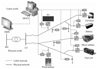
Ⅱ. CYBER PHYSICAL ENERGY SYSTEM FOR MICROGRID ENERGY MANAGEMENTThe architecture of CPES for microgrid energy management is shown in Fig. 1. The CPES is a combination of the physical world and cyber world in microgrid.
|
Download:
|
| Fig. 1. Configuration of a typical microgrid CPES system. | |
In the physical world,distributed energy sources (DECs) in the household or community,including PVs,WTs,fuel cells (FCs) and storage units (battery banks) generate electricity to supply local customer loads through low level transmission lines. Through the power electronic interfaces and real time smart controls,the DECs and customer loads are connected to low level transmission lines forming the physical system of a microgrid. The microgrid is operated in either grid-connected mode or islanded mode,and the bidirectional power flow is admitted. The dynamic (frequency and voltage) or static (power flow) physical processes are major concerns because these processes have a large impact on system performance in the aspects of security,reliability and economy.
In the cyber world,the system performances are monitored and controlled to execute stable and optimal operation of the MG through a communication network,like wired/wireless network of sensor/actuator arrays,WLAN,Bluetooth,GSM,etc[6]. The centralized microgrid control architecture generally consists of three control levels: local control (LC) level at individual DERs,MG central control (MGCC) level,and distribution management system (DMS) level[12]. The LC uses real-time local information to control the voltage and the frequency of the microgrid in transient conditions[11]. The MGCC is responsible for the optimal control and operation of the microgrid. It uses the real time and historical data of the intermittent DERs (PVs and WTs) and loads to predict the future supply and demands,then make scheduling plan to operate microgrid in an economic manner. The DMS is in charge of the power exchange between MGs and the grid.
The performance of microgrid management system depends on the accuracy of prediction on intermittent DERs generation and customer loads. However,randomness in physical world such as the change of the weather,human preference as well as error in sampling/measurement will definitely have a significant influence on the results of the prediction. Now,probability and statistics have taught us that the future cannot be perfectly forecasted but instead should be considered in a random or uncertain framework. This requires a novel decision scheme considering uncertainties,which will be described in more detail in Section III. The decision scheme is assumed to be able to improve the efficient performance because it is based on appropriate modeling strategy on the uncertainties. In addition,the dynamic and steady-state security of the microgrid system such as voltage constraints and power flows limits are not in the scope of our discussion.
Ⅲ. STOCHASTIC PROGRAMMING BASED MICROGRID ENERGY OPTIMAL OPERATION A. Introduction to Two-stage Stochastic ProgrammingStochastic programming is a flexible and effective modeling method that can incorporate a high degree of uncertainty. Two-stage with recourse problem as a general problem in stochastic programming is well suited to model MGs optimal scheduling problem. The classical two-stage with recourse stochastic programming problem can be described as follow[13, 14].
| \[\min \;z = {c^{\rm{T}}}x + {E_\xi }[\min q{(\omega )^{\rm{T}}}y(\omega )],\] | (1) |
| \[{\rm{s}}.{\rm{t}}.\;\;Ax = b,\] | (2) |
| \[T(\omega )x + Wy(\omega ) = h(\omega ),\] | (3) |
| \[x \ge 0,\;y(\omega ) \ge 0.\] | (4) |
As shown in the objective function (1),it consists of a deterministic term $c^{\rm T}{ x}$ and the expectation of the second-stage objective ${ q}(\omega)^{\rm T}{ y}(\omega)$ taken over all realizations of the random event $\omega$. The decisions are split into two different stages depending on the different moments of decisions. The vector ${ x}$ represents all the first-stage decisions that have to be taken before the random experiment. The vector ${ y}(\omega)$ is the second-stage decisions that have to be taken after the random experiment. Corresponding to two different stages,(2) and (3) hold the first-stage constraint and the second-stage constraint respectively. Here,$\omega$ is a possible realization of the random variable $ \xi(\omega)$ defined over probability space $( \Omega,{ P})$.
B. Modeling for Microgrid Energy Optimal OperationIn this section,we focus on the decision process in micro grid control center (MGCC),and formulate optimal operation decision model. To a great extent,the optimal scheduling decisions for a microgrid depends on the future information about renewable generation and demand loads. However,the randomness in the physical world is extremely hard to capture by the cyber world. Therefore,the modeling strategy in the cyber world should be considered by combining the physical world proceeding in random or uncertain frame.
In our model,the uncertainties of WT generation,PV generation,load demands are considered in the optimal operation problem of the MG. In an open electricity market,the MGCC must make decisions (first-stage decisions) about how much electricity it will purchase from each distributed generator (DG) and utility in advance. However,since the WTs generation,PVs generation and users loads are random,there has to be a gap between demand and supply in reality. For security needs,the gap will be filled with storage units or spinning reserves (second-stage decisions) which are very expensive. In order to reduce operational cost of MG,the first-stage decisions the MGCC makes must try to keep the gap as small as possible so as to minimize the cost of energy storage and spinning reserves.
1) Objective: The optimization goal is to minimize the operation cost of the MG over the prediction horizon under the condition of uncertainty. According to the above analysis,the operation cost consists of two parts: the first-stage cost includes the cost of electricity purchased in advance and units start-up costs; the second-stage cost is the expected cost of the sum of electricity purchased from spinning reserves and energy storage costs. Positive electricity purchase cost means purchasing electricity from utility grid and negative electricity cost means selling electricity to utility grid. When the MG is running in the islanding model,the electricity purchase cost is 0. The objective function is given in (5).
| \begin{align} &\min\,f=\sum_{t=1}^T\sum_{i=1}^I\left(p_i^tb_i^t+C_i^t+p_{\rm grid}^tb_{\rm grid}^t\right) \Delta t \notag \\%c^{T}x+E_{ \xi}[\min q(\omega)^Ty(\omega)]\times\label{1}\\ &\ \ +\min\,E_{ \xi}\left[\sum_{t=1}^T\sum_{j=1}^J \left( \lvert p_{rs}^t(\omega)\rvert b_{rs}^t(\omega)+\lvert p_j^t(\omega)\rvert b_j^t(\omega) \right)\Delta t \right], \end{align} | (5) |
where $p_i^t$ and $p_{\rm grid}^t$ are the first-stage decision variables,which represent the amount of electricity purchase from the $i$-th DG and from the utility at hour $t$ respectively. The first-stage decision variables must be made in advance,so the cost is free from random factors. $p_{\rm grid}^t$ can be either positive which means purchasing electricity from utility or negative which means selling electricity to utility. $C_i^t$ represents the sum of the hourly payback amount for the investment and the start-up/shut-down cost of the $i$-th unit. $b_i^t$ and $b_{\rm grid}^t$ are the bids of the $i$-th DG and the utility per kWh respectively. $p_{rs}^t(\omega)$ and $p_j^t(\omega)$ are the second-stage decision variables,which represent the output power spinning reserves and the $j$-th storage unit at hour $t$ respectively. They have to be decide according to the realizations of all random events. Notice that $p_{rs}^t(\omega)$ can be either positive when the supply cannot meet the demands or negative when there exists surplus supply. Both cases can lead to extra costs to spinning reserves. Similar to the storage units,frequent charging and discharging cause the degradation of storage units,where $b_{rs}^t(\omega)$ and $b_j^t(\omega)$ represent the cost of the spinning reserves and the degradation cost of the $j$-th storage units per kWh respectively. $\Delta t$ is a constant and indicates the time interval $\left[t-1,t\right)$ for any $t\in T$.
2) Constraints: At any moment,the total power generation and the total demand loads should keep balance.
| \begin{align} \sum_{i=1}^Ip_i^t+p_{\rm grid}^t+p_{rs}^t(\omega)=\sum_{j=1}^Jp_j^t+p_{\rm load}^t,\ \ t=1,2,\ldots,T, \end{align} | (6) |
where $p_{\rm load}^t$ is the aggregated average user loads units at hour $t$ respectively. They are all modeled as random variables with certain distribution.
The output power of all distributed generation units is limited to a certain range because of technical reasons.
| \[P_i^{{\rm{min}}} \le p_i^t \le P_i^{{\rm{max}}},\] | (7) |
| \[- P_j^{{\rm{discharge}},{\rm{max}}} \le p_j^t(\omega ) \le P_j^{{\rm{charge}},{\rm{max}}},\] | (8) |
where $p_i^{\rm min}$ and $p_i^{\rm max}$ are the minimum and maximum output power of the $i$-th DG,$p_j^{{\rm charge},{\rm max}}$ and $p_j^{{\rm discharge},{\rm max}}$ are the maximum charge and discharge power of the $j$-th storage unit.
The remaining capacity of the $j$-th storage unit $e_j^t$ is constrained to avoid over-charging or over-discharging within (9). Energy conservation equation considering conversion efficiency and the self-discharging rate is given by (10).
| \[E_j^{{\rm{min}}} \le e_j^t \le E_j^{{\rm{max}}},\] | (9) |
| \[e_j^t = \lambda _j^{{\rm{self}}}e_j^{t - 1} + [\eta _j^{{\rm{char}}}\max (0,p_j^t(\omega ) + \eta _j^{{\rm{dis}}}\max \left( {0,- p_j^t(\omega )} \right)]\Delta t,\] | (10) |
where $E_j^{\rm min}$ and $E_j^{\rm max}$ are respectively the lower bound and upper bound of energy storage for the $j$-th storage unit. Where $\lambda_j^{\rm self}$ is the self-discharging rate of the $j$-th storage unit,and $\eta _j^{\rm char}$/$\eta _j^{\rm dis}$ are the charging/discharging efficiency of the $j$-th storage unit.
C. Scenarios-based Uncertainties ModelingSolving the formulations given in Section III-B is an extremely cumbersome even impossible job because it requires high dimensional integral operation corresponding to the continuous random variable $\xi(\omega)$ to calculate the expected value of the second stage. A practical method to solve the problem is to consider the approximation of the original problem by taking $n$ samples $\omega(s)$,$s=1,2,\ldots,n$ from sample space $ \Omega$ of random variable $ \xi(\omega)$ according to its distribution. Each sample corresponds to a possible realization which is represented by a scenario with a certain probability. In this way,we can decompose the complex two-stage stochastic programming problem into $n$ easy-to-solve deterministic mixed integrated linear programming (MILP) subproblems with different probabilities by minimizing the expectation of the $n$ subproblems. The approximation problem is expressed as (11).
| \begin{align} \min\ \sum_{s=1}^n\pi_sf(\omega(s)). \end{align} | (11) |
The first step to approximate the stochastic programming model is to know the probabilistic characteristics of the random variables,which often mean WTs and PVs production as well as loads in a MG. Unfortunately,it is very hard to find out their probabilistic characteristics since they involve too many random factors,like illumination intensity,cloud cover,temperature variations,etc. However,it should be noted that the uncertainties can essentially be depicted as a form of the forecast errors of WTs and PVs power production as well as loads,and with these factors it is easy to execute a statistical analysis. We use random variables $ \xi_{wt}(e_{wt})$,$ \xi_{pv}(e_{pv})$ and $ \xi_{\rm load}(e_{\rm load})$ to indicate the forecast errors of the WTs production,PVs production and loads respectively. According to Section III-B,the second-stage decisions $p_{rs}^t(\omega)$ and $p_j^t(\omega)$ are used to fill the gap between supply and demand caused by uncertainties,so they can be expressed as (12).
| \begin{align} & p_{rs}^t(e_{wt},e_{pv},e_{\rm load})-p_{j}^t(e_{wt},e_{pv},e_{\rm load}) \notag \\ &\quad={ \xi}_{wt}(e_{wt})+{ \xi}_{pv}(e_{pv})+{ \xi}_{\rm load}(e_{\rm load}) .\label{12} \end{align} | (12) |
Therefore,the second-stage decisions $p_{rs}^t(e_{wt},e_{pv},e_{\rm load})$ and $p_{j}^t(e_{wt},e_{pv},e_{\rm load})$ become related to random variables ${ \xi}_{wt}(e_{wt})$,${ \xi}_{pv}(e_{pv})$ and ${ \xi}_{\rm load}(e_{\rm load})$. For random variables ${ \xi}_{wt}(e_{wt})$ and ${ \xi}_{pv}(e_{pv})$,they are assumed to follow a normal distribution ${\rm N}(\mu,\sigma^2)$. The load forecast error ${ \xi}_{\rm load}(e_{\rm load})$ is assumed to fit the truncated normal distribution (TND) according to [15]. The probability density function (PDF) of the truncated normal distribution is formulated in (13).
| \begin{align} & PDF_{TND}(x,\mu,\sigma,a,b) \notag \\ &\quad\ =\frac{\frac{1}{\sigma}PDF_N \left(\frac{x-\mu}{\sigma} \right)} {CDF_N \left(\frac{b-\mu}{\sigma}\right)-CDF_N \left(\frac{a-\mu}{\sigma} \right)}, \end{align} | (13) |
where $\mu$,$\sigma$,$a$,$b$ are the mean value,the standard deviation,upper and lower limits of the non-truncated normal distribution respectively. $CDF_N(\cdot)$ is the cumulative distribution function (CDF) of the standard normal distribution.
Once the probability distributions of these random variables are known,we will be able to apply a method of discretization to solve the stochastic programming model approximately. The main idea is to use samples or scenarios to represent possible states of physical world in the future,as the preceding description. As a result,the uncertainty in the physical world can be simulated via discrete scenarios and then be analyzed and calculated easily in the cyber world. It should be noted that a rational and effective scenarios generation method is the key to simulate the uncertainty of real world. It helps expose the effects of physical world on cyber world.
The autoregressive moving average (ARMA) models based on time series theory is used to generate time-series-based scenarios. This is because that the forecast error during scheduling period is essentially a time series and correlated in time. It is reasonable and easy to model it as a stochastic process and simulate it by scenarios in a way of time series over the scheduling period. An $ARMA(p,q)$ series can be expressed as (14).
| \begin{align} y_{t}=\sum_{i=1}^p \phi_i y_{t-i}+\varepsilon_t-\sum_{i=1}^q \theta_i\varepsilon_{t-1},\label{14} \end{align} | (14) |
where $\varepsilon_t$ is a white noise series,and $p$ and $q$ are nonnegative integers which mean the order of $AR(p)$ and $MA(q)$ respectively. The choice of the order of ARMA model depends on auto-correlation function (ACF) and partial ACF (PACF) of sample data. The scenarios generation process based on $ARMA(p,q)$ model is described as follow. First,we apply the $ARMA(p,q)$ to get a time series over scheduling period,which is in terms of white noise and follows normal distribution. In the process,the probability of each value in the time series is obtained. Second,the time series is transferred to another time series,which follows the distribution of forecast error of WTs production,PVs production or loads as needed,via distribution transformation. The transformation function is mathematically expressed as (15).
| \begin{align} Z={ \Phi}^{-1}\left[F(y)\right],\label{15} \end{align} | (15) |
where $F(y)$ is the CDF of the generated time series by ARMA model and ${ \Phi}^{-1}(\cdot)$ is the inverse of cumulative distribution function (CDF) of the corresponding forecast error random variable. The new time series $Z$ is just a corresponding random scenario of forecast error. Then,repeat the process until getting enough scenarios.
Although substantial scenarios bring a more precise approximation on continuous distribution,a dilemma is that a large number of scenarios cause computational difficulties. A wise balance is by reducing some scenarios from the set of massive scenarios while keeping the original probability characteristics as much as possible. The basic idea of scenario reduction is to remove scenarios with very low probability and those that are similar to another one. In our study,a scenario reduction strategy proposed by [16] is adopted,and detailed description is given as follow.
Let $n$ denotes the number of the scenarios,and the probability of each scenario ${ S}_i$,$i=(1,2,\ldots,n)$ is denoted as $\pi_i$. Here,${ S}_i$ is a vector with $m$ elements. Assume that the number of scenarios is expected to reduce to $N$. Let the distance between two scenarios $\mu_i$ and $\mu_j$ is described as a 2-norm.
| \begin{align} d\left({ S}_i,{ S}_j\right)=\Vert { S}_i-{ S}_j \Vert. \label{16} \end{align} | (16) |
Then,the scenarios reduction algorithm is implemented iteratively until a given number of scenarios $N$ is remaining.
Algorithm 1. The scenarios reduction
1. procedure scenarios reduction (${ S}$,$\pi$,$d$)
2. while $n>N$ do
3. ${\rm remove\ scenario}\ { S}_r\ {\rm satisfying:}$
4. ${\pi _r} \cdot \mathop {\min }\limits_{r \ne i} d({{ S}_r},{{ S}_i}) = \mathop {\min }\limits_{k \in (1,2,\ldots,n)} {\pi _k} \cdot \mathop {\min }\limits_{k \ne j} d({{ S}_k},{{ S}_j})$
5. $n\gets n-1 $
6. $\pi_{r^*}\gets \pi_{r^*}+\pi_{r}$
7. end while
8. end procedure
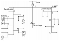
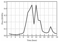
IV. CASE DESCRIPTIONThe proposed modeling method for microgrid energy management is applied on a modified low voltage (LV) network from [11],shown in Fig. 2,for one day. The MGCC operates the MG every 15 minutes according to the scheduling plans from 00 : 00 to 24 : 00. The network includes three feeders which separately serve a primarily residential area,a workshop and a commercial consumer. A wide variety of DGs including a micro turbine (MT),a proton exchange membrane fuel cell (PEM-FC),storage device (NiMH battery),a small-scale WT and PVs are installed in the MG. The maximum and the minimum operating limits of each DG are shown in Table I. Also,the bids of all DGs and their start-up cost are presented in the same table. The bids of spinning reserves $b_rs^t$ is assumed to be 0.25 /kWh and the day-ahead grid electricity price is depicted in Fig. 3. For simplicity,all DGs are assumed to be working at unity power factor and there is no reactive power exchange.
|
Download:
|
| Fig. 2. LV network study case for MG. | |
|
Download:
|
| Fig. 3. Day-ahead grid electricity price. | |
|
|
Table I LIMITS AND BIDS OF THE INSTALLED |
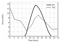
The forecast values of the WT and PV generation for the next 24 hours in the MG are shown in Fig. 4. They are based on the day-ahead forecast data of WT and PV production on September $1$,$2014$ in Belgium provided by ELIA[17]. Since the data is obtained from a large high voltage power grid,appropriate normalizations are made to match the level of the MG. The data is recorded as a form of time series over 15 minute intervals,so there are 96 data points of each of the PV and WT production forecasts. According to Section III-C,the uncertainties in the PV and WT production are depicted by the form of prediction error with normal distribution. In order to estimate the distribution parameters,the statistical prediction error data,of both the PV and WT production over the course of a year between September $1$,$2013$ and August 31,2014 in Belgium from ELIA is normalized and then analyzed. Matlab distribution fitting toolbox is employed to implement the process. It turns out that the forecast errors of the PV follow normal distribution with the mean value of $-0.39$ and the standard deviation of 1.065. The mean value and standard deviation for the forecast errors of WT production are $-0.33$ and 1.35.
|
Download:
|
| Fig. 4. Day-ahead forecast curve of WT and PV production. | |
It is assumed that the aggregated load demand for the next day equals 1 943 kWh. In our study,all loads are supposed to be active loads. The predicted total energy demand data (from ELIA) in Belgium on the same day is adapted. In order to match the scale of the PV and WT generation,the same normalized process mentioned before is used. The forecasted load demands curve is shown in Fig. 5. Similarly,the distribution parameters of the load forecast errors are estimated based on the statistical data of load forecast errors (from ELIA) in Belgium over the course of a year between September 1,$2013$ and August 31,$2014$. It turns out that the load forecast errors follow TND with the mean value of $-2.88$ and the standard deviation of 5.92.
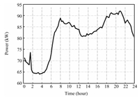
|
Download:
|
| Fig. 5. Forecasted load demands curve. | |
According to the distribution of the forecast errors in WT generation,PV generation and load,scenarios generation method mentioned in Section III-C is used to depict their randomness. In order to reveal the advantage of the proposed stochastic programming model,the optimization problem is first solved by deterministic approach for the purpose of comparison. The simulations are carried out on an Intel (R) Core (TM) i5-2400,3.10 GHz personal computer with 4 GB RAM memory. The simulation tool is Matlab R2012b.
A. Results of Deterministic MethodIn this subsection,we solve the energy optimization operation of MGs by the deterministic method in which the random variables are replaced by their forecasted time series values. The results obtained from the deterministic method show that the anticipated operating cost for the next day is 96.403. The optimal scheduling of all the units is shown in Fig. 6. As shown in this figure,during 00 : 00 to 7 : 00,the market electricity prices are favorable,so the MGCC purchases active power from main grid as much as possible. As the market electricity prices go up after 7 : 00,electricity purchased from main grid dramatically decreases. Meanwhile,more electricity is imported from DGs to meet user loads. From 8 : 00 to 16 : 00,major electricity supply comes from FC and MT and part of the surplus electricity is sold to the utility for profits. Noticeably,as the market bid goes down at 16 : 00,the power production of MT decreases significantly for its cost advantage has diminished,but FC still works because it is much cheaper.
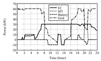
|
Download:
|
| Fig. 6. Optimal power production schedule based on deterministic method. | |
In addition,the initial state of charge (SOC) of battery is assumed to be empty,so it has to be charged (positive power output) so as to be able to be discharged (positive power output) during peak hours at the beginning. From Fig. 6,it can be seen that the battery starts to charge itself for 3 hours after midnight and then discharges between 9 : 00 and 12 : 00. This is because that the load is low after the midnight and peaks in the morning. In fact,the usage of battery helps improve load-generation matching and hence leads to a lower energy cost.
B. Results of Proposed Stochastic MethodOne disadvantage of deterministic method is the lack of robustness. Although it works well when the forecast is precise,it usually cannot obtain good performance in reality because of the hard-to-capture uncertainties. To overcome the problem,the proposed two-stage stochastic programming model is applied to find a favorable scheduling solution which is expected to balance the various uncertainties. In the stochastic model,the uncertainties are handled by using the expected value of the second stage instead of their forecasted values,and then the stochastic problem is decomposed into deterministic problem. In order to lower the computational cost,the scenario simulation method mentioned in Section III-C is implemented. 1 000 stochastic scenarios are generated first and then reduced to 10 scenarios. The anticipated operating cost for the next day is 100.69. The scheduling of all the units obtained from the proposed stochastic model is shown in Fig. 7. From the anticipated results,it seems that the deterministic method is much better because it can obtain a lower operating cost. However,the cost is only an anticipated cost but not a real operating cost occurring in the physical world. So,it is too early to conclude that the deterministic method outperforms the proposed stochastic method.
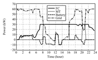
|
Download:
|
| Fig. 7. Optimal power production schedule based on stochastic method. | |
In order to reveal the advantage of the stochastic model,we compare the results of optimization from deterministic method and stochastic method. Real WT and PV production as well as real demand loads on September 1,$2014$ in Belgium provided by ELIA are used to calculate the real cost of each method based on their scheduling decisions. In order to compare with the forecast data,the same data processing method was used. The real data is listed in Table II.
|
|
Table II WT, PV PRODUCTION AND LOADS REAL DATA |
The anticipated and real operation cost obtained from stochastic method and deterministic method are given in Table III. The result shows that the real cost obtained from deterministic method is 252.12. That is too much higher than 169.85,which is the real cost obtained from stochastic method. The increased cost is due to the uncertainties that need expensive spinning reserves to mitigate real time imbalance. Once there are big forecast errors,the real operating cost will increase drastically. The optimization solution is very sensitive to variations in the prediction of random variables. On the contrary,the stochastic programming method can provide MGCC with a more robust scheduling plans even though the plans are not optimal. But it can thus minimize the risk from the impact of uncertainties and reduce its cost. This is because the consideration of uncertainties helps MGCC judge and weigh the cost and risk so that it can obtain a good hedging against various uncertainties.
|
|
Table III MG OPERATION COST OBTAINED FROM DETERMINISTIC METHOD AND STOCHASTIC METHOD |
This paper focuses on the randomness in physical world of microgrid CPES and its effects on the energy optimization operation decision making process. The goal is to reduce the energy costs of MGs in the long run. The proposed energy scheduling optimization strategy for MGs is based on two-stage stochastic program by considering uncertainties in microgrid CPES. The uncertainties are modeled by generating stochastic scenarios according to PDF of each random variable. The simulation result shows that the proposed stochastic programming model possesses a good characteristic of finding robust solutions which are able to make hedging against various uncertainties and minimizes the expected energy cost of the microgrid. Consequently,the proposed energy scheduling optimization strategy can provide a robust and favorable energy scheduling solution for MGs under uncertain operating environment.
| [1] | Ilic M D, Xie L, Khan U A, Moura J M F. Modeling of future cyber physical energy systems for distributed sensing and control. IEEE Transactions on Systems, Man, and Cybernetics, Part A:Systems and Humans, 2010, 40(4):825-838 |
| [2] | Palensky P, Widl E, Elsheikh A. Simulating cyber-physical energy systems:challenges, tools and methods. IEEE Transactions on Systems, Man, and Cybernetics:Systems, 2014, 44(3):318-326 |
| [3] | Ge Y Q, Dong Y W, Zhao H B. A cyber-physical energy system architecture for electric vehicles charging application. In:Proceedings of the 12th International Conference on Quality Software (QSIC). Xi'an, China:IEEE, 2012. 246-250 |
| [4] | Jamshidi M M. Sustainable energy systems:cyber-physical based intelligent management of micro-grids. In:Proceedings of the 4th IEEE International Symposium on Logistics and Industrial Informatics (LINDI). Smolenice:IEEE, 2012. 11-12 |
| [5] | Macana C A, Quijano N, Mojica-Nava E. A survey on cyber physical energy systems and their applications on smart grids. In:Proceedings of the 2011 IEEE PES Conference on Innovative Smart Grid Technologies (ISGT Latin America). Medellin:IEEE, 2011. 1-7 |
| [6] | Susuki Y, Koo T, Ebina H, Yamazaki T, Ochi T, Uemura T, Hikihara T. A hybrid system approach to the analysis and design of power grid dynamic performance. Proceedings of the IEEE, 2012, 100(1):225-239 |
| [7] | Chakraborty S, Weiss M D, Simoes M G. Distributed intelligent energy management system for a single-phase high-frequency AC microgrid. IEEE Transactions on Industrial Electronics, 2007, 54(1):97-109 |
| [8] | Chen C, Duan S, Cai T, Liu B, Hu G. Smart energy management system for optimal microgrid economic operation. Renewable Power Generation, IET, 2011, 5(3):258-267 |
| [9] | Kriett P O, Salani M. Optimal control of a residential microgrid. Energy, 2012, 42(1):321-330 |
| [10] | Ahn S J, Nam S R, Choi J H, Moon S I. Power scheduling of distributed generators for economic and stable operation of a microgrid. IEEE Transactions on Smart Grid, 2013, 4(1):398-405 |
| [11] | Tsikalakis A G, Hatziargyriou N D. Centralized control for optimizing microgrids operation. In:Proceedings of the 2011 IEEE Power and Energy Society General Meeting. San Diego, CA:IEEE, 2011. 1-8 |
| [12] | Zhang D, Li S H, Zeng P, Zang C Z. Optimal microgrid control and power-flow study with different bidding policies by using powerworld simulator. IEEE Transactions on Sustainable Energy, 2014, 5(1):282-292 |
| [13] | Birge J R, Louveaux F. Introduction to stochastic programming. Springer Series in Operations Research and Financial Engineering. New York:Springer-Verlag, 1997. |
| [14] | Deng R L, Yang Z Y, Chen J M, Chow M Y. Load scheduling with price uncertainty and temporally-coupled constraints in smart grids. IEEE Transactions on Power Systems, 2014, 29(6):2823-2834 |
| [15] | Members of Renewables Workgroup California Independent System Operator Corporation. Integration of renewable resources[Online], available:http://www.caiso.com/1ca5/1ca5a7a026270.pdf, November 1, 2007. |
| [16] | Dupačová J, Gröwe-Kuska N, Römisch W. Scenario reduction in stochastic programming:an approach using probability metrics. Mathematical Programming, Series B, 2003, 95(3):493-511 |
| [17] | The ELIA. Belgiums electricity transmission system operator website[Online], available:http://www.elia.be/, September 1, 2014. |
 2015, Vol.2


