2. School of Mathematics & Physics, Qingdao University of Science & Technology, Qingdao 266061, China;
3. College of Automation & Electronic Engineering, Qingdao University of Science & Technology, Qingdao 266042, China;
4. School of Mathematics & Physics, Qingdao University of Science & Technology, Qingdao 266061, China
THE key factor for the future planetary landing missions is the onboard autonomy,particularly in the relevant missions towards planets at high distances from Earth. As an example,the travel time of a radio frequency signal requires 4 to 22 minutes to cover the distance between the Earth and Mars. When landing on Mars,for example,non-zero steady state winds could effect horizontal velocity at impact,which might burst the airbags or the lander[1, 2]. So the horizontal velocity could be reduced by firing the retro-rockets into the wind using transverse impulse rockets system (TIRS) prior to landing. However,the error in position due to a bias in the accelerometer will have quadratic growth with time,and the errors in misalignment of the accelerometer axes will propagate into position errors as well. In order to provide accurate estimates of the lander position and velocity,a tightly coupled estimation process is employed to use features observable from a camera,such as the descriptions of some early works[3, 4]. Descent image motion estimation system (DIMES)[5],developed by NASA,can be considered as the first historical attempt to exploit computer vision to control a spacecraft during the entry,decent,landing (EDL) phase. DIMES software tracked all of the features correctly,but discarded the second feature of the second image pair,because the Harris operator[6] was not scale invariant and sensitive to noise. Recently,several studies have shown various visual techniques to estimate position and velocity parameters[7, 8, 9, 10]. However,many recent advanced results from the field of computer vision were achieved,thanks to the availability of high computational power,but were often not able to meet the hard real-time performance[11, 12, 13].
By tracking multiple features and applying checks on feature correlation across two images,a novel approach of direct horizontal velocity estimation is employed. This method is real-time and low-computational. It can be used to land on the planet without relying on a map or some known features of the ground. Compared with the algorithm of DIMES,the proposed method is more accurate and has lower complexity than the above-mentioned algorithms in the literature.
Note that there is another significant problem before the horizontal velocity is estimated. That is,the feature points have to be selected inside the overlap among at least two successive images. Because of the complexity of the planetary environment (such as Mars weather),the trajectories may have stronger winds and consequently greater horizontal velocity and attitude excursions. Then the cases of very small overlap or nonoverlap area between the adjacent field of views (FOVs) may usually occur when matching feature points in different images. So the velocity cannot be estimated due to lack of correspondence between two images. Therefore,with the limited FOVs of the navigation camera,and the low frame rates,it is necessary to get the relationship between overlapping area and the camera motion. The computations of the field of view lines (FOV lines) are essentially the edges of the footprint,which help us establish correspondence between trajectories.
The paper is organized as follows. In Section Ⅱ,the camera model and the overlapping area formulas as well as the motion constraints of planetary lander with overlapping FOVs are illustrated. Section Ⅲ provides a discussion of the horizontal velocity estimation based on the least square method. Finally some conclusions are drawn in Section Ⅳ.
Ⅱ. OVERLAPPING AREA REPRESENTATIONFinding the intersected polygons and computing the overlapped areas is the key issue to feature tracking. In order to prevent gaps from occurring due to crab,tilt and flying height variations,the amount of overlapping is normally greater than 50 %. So,before computing the horizontal velocity of lander,the relationship between the overlapping area and the movement of lander must be found.
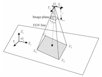
A. The Camera ModelThe camera rig mounted on the planetary lander produces a 2D image by using a projection transformation of the landing site scene. In this paper,a pin-hole model is used to describe the geometry of camera imaging principles,as shown in Fig. 1. The camera coordinate system $O_c-X_cY_cZ_c$ fixed relative to the spacecraft body frame is established as follows. The center of camera O$_{c}$ is considered as the origin of the camera coordinates. The Z$_{c}$ axis is coinciding with the optical axis and points toward the ground. The X$_{c}$ axis points in the direction of the scan. The Y$_{c}$ axis completes the right-handed orthogonal coordinate system and is parallel to the long axis of the detector arrays. $\gamma$ is the camera$'$s angle of view measured diagonally. The origin of image coordinates O$_{i}$ is the intersection point of principle axis and image plane. The image plane is parallel to axes $X_{c}$ and $Y_{c}$,and is located at distance $f$ from the origin $O_{c}$.
|
Download:
|
| Fig. 1. Camera model and its coordinate system. | |
Any feature point P$_c$ in the camera coordinate system can be expressed by
| ${P_c} = \left[\begin{array}{l} {X_c}\\ {Y_c}\\ {Z_c} \end{array} \right] = - RC + R\left[\begin{array}{l} {X_L}\\ {Y_L}\\ {Z_L} \end{array} \right]$ | (1) |
where ${ C}=[C_x$ $C_y$ $C_z$]$\rm ^T$ is the lander position in the landing site cartographic coordinate system,its posture is represented by a rotation matrix ${R}$,[$X_L$ $Y_L$ $Z_L$]$\rm ^T$ are coordinates of the feature points described in landing site cartographic coordinate system $O_{L}-X_{L}Y_{L}Z_{L}$. The point corresponding to point ${ P}_c$ in the 2D image plane coordinate is denoted as ${ p}=[u,v]^{\rm T}$. The relationship of these two coordinates systems is given by
| ${Z_c}\left[{\begin{array}{*{20}{c}} u\\ v\\ 1 \end{array}} \right] = \left[{\begin{array}{*{20}{c}} {{f_x}}&0&{{c_x}}&0\\ 0&{{f_y}}&{{c_y}}&0\\ 0&0&1&0 \end{array}} \right]\left[{\begin{array}{*{20}{c}} {{X_c}}\\ {{Y_c}}\\ {{Z_c}}\\ 1 \end{array}} \right],$ | (2) |
where (c$_{x}$,c$_{y}$) are the coordinates of image center O$_{i}$,f$_{x}$ and f$_{y}$ are the local lengths along the x axis and y axis,respectively.
Radial lens distortion is the dominant distortion in the descent imagery. The observed focal plane coordinates ( u$'$,v$'$) are then assumed to be related to the ideal coordinates (u,v) by a purely radial transformation
| $\begin{array}{l} \frac{{u'}}{{r'}} = \frac{u}{r},\\ \frac{{v'}}{{r'}} = \frac{v}{r}, \end{array}$ | (3) |
where
| $\begin{array}{l} r' = \sqrt {{{u'}^2} + {{v'}^2}} ,\\ r{\rm{ }} = \sqrt {{u^2} + {v^2}} . \end{array}$ | (4) |
Finally,the distortion $\Delta r=r'-r$ is modeled by a polynomial of the form
| $\Delta r = {k_0}r + {k_1}{r^3} + \cdots .{\rm{ }}$ | (5) |
In order to consistently tracking feature points,the relations between adjacent cameras should be first estimated offline by finding the limits of FOV of a camera as visible in the other cameras. The FOV of the $i{\rm th}$ camera is a rectangular pyramid in the space. The intersections of FOV lines with the ground plane are denoted as $L_1^i,~L_2^i,~L_3^i$ and $L_4^i$ (Fig. 1). As far as the camera pair $i,i+1$ are concerned,the only locations of interest in the two images for handoff are $L_j^i$ and $L_j^{i+1}~(j\in\{1,2,3,4\})$.
B. Pure 3D TranslationWith the assumption that the landing region is approximately flat compared to the height of the camera,so the algorithm does not need to account for depth of features. Generally,the lander flies over the area to be photographed and takes a series of images,each of which overlaps the preceding image and the following image,so that an unbroken coverage of the area is obtained. In this case,all that needs to be done is to compute whether the FOV associated lines in the two images cross each other or not.
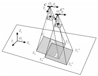
Some assumptions are used in order to simplify computational processes so that they are easier to be represented. Assume that the initial position of the lander in the landing site cartographic coordinate system is ${ C}=[C_x$ $C_y$ $C_z$]$\rm ^T$,its $Z_c$ axis is perpendicular to the ground,its axes $X_c$ and $Y_c$ are parallel to the axes $X_L$ and $Y_L$,respectively,and the shear deformations will be neglected. After taking a movement $\Delta C=\begin{bmatrix}\Delta C_x & \Delta C_y & -\Delta C_z \end{bmatrix} \rm^T $ $(\Delta C_z>0)$ without any attitude change,its position becomes $ C'= C + \Delta C = \begin{bmatrix} C_x' & C_y' & C_z'\end{bmatrix} \rm ^T$ (Fig. 2).
|
Download:
|
| Fig. 2. 3D translation scenario of camera pair. | |
Using projection formula,the four coordinates of $L_1^i,~L_2^i,~L_3^i$ and $L_4^i$ limited by FOVs on the landing site plane can be easily derived,which are
$\left( {\frac{{{C_z}}}{{\sqrt 2 }}\tan \frac{\gamma }{2} + {C_x},\frac{{{C_z}}}{{\sqrt 2 }}\tan \frac{\gamma }{2} + {C_y}} \right),$
$\left( { - \frac{{{C_z}}}{{\sqrt 2 }}\tan \frac{\gamma }{2} + {C_x},\frac{{{C_z}}}{{\sqrt 2 }}\tan \frac{\gamma }{2} + {C_y}} \right),$
$\left( { - \frac{{{C_z}}}{{\sqrt 2 }}\tan \frac{\gamma }{2} + {C_x},- \frac{{{C_z}}}{{\sqrt 2 }}\tan \frac{\gamma }{2} + {C_y}} \right),$
$\left( {\frac{{{C_z}}}{{\sqrt 2 }}\tan \frac{\gamma }{2} + {C_x},- \frac{{{C_z}}}{{\sqrt 2 }}\tan \frac{\gamma }{2} + {C_y}} \right).$
The ground plane coordinates of {$L_j^{i+1}(j\in\{1,2,3,4\})$} can be obtained similarly. The following discussion will analyze overlapping area between two rectangles in 5 different cases.
1) If the translations in $x$ direction and $y$ direction satisfy condition (6),i.e.,
| $\begin{array}{l} \frac{{\Delta {C_z}}}{{\sqrt 2 }}\tan \frac{\gamma }{2} < |\Delta {C_x}| < \frac{{2{C_z} - \Delta {C_z}}}{{\sqrt 2 }}\tan \frac{\gamma }{2},\\ \frac{{\Delta {C_z}}}{{\sqrt 2 }}\tan \frac{\gamma }{2} < |\Delta {C_y}| < \frac{{2{C_z} - \Delta {C_z}}}{{\sqrt 2 }}\tan \frac{\gamma }{2}, \end{array}$ | (6) |
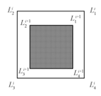
the overlapping rectangle corresponding to the two FOVs are shown in Fig. 3.

|
Download:
|
| Fig. 3. Overlapping region in Case 1. | |
The area of the overlapping rectangle is given by
| $\begin{array}{l} S = \left( {\frac{{2{C_z} - \Delta {C_z}}}{{\sqrt 2 }}\tan \frac{\gamma }{2} - |\Delta {C_x}|} \right) \times \\ \left( {\frac{{2{C_z} - \Delta {C_z}}}{{\sqrt 2 }}\tan \frac{\gamma }{2} - |\Delta {C_y}|} \right). \end{array}$ | (7) |
2) If the translations in $x$ direction and $y$ direction satisfy condition (8),i.e.,
| $\begin{array}{l} |\Delta {C_x}| < \frac{{\Delta {C_z}}}{{\sqrt 2 }}\tan \frac{\gamma }{2},\\ \frac{{\Delta {C_z}}}{{\sqrt 2 }}\tan \frac{\gamma }{2} < |\Delta {C_y}| < \frac{{2{C_z} - \Delta {C_z}}}{{\sqrt 2 }}\tan \frac{\gamma }{2}, \end{array}$ | (8) |
the overlapping rectangle corresponding to the two FOVs can be shown in Fig. 4.

|
Download:
|
| Fig. 4. Overlapping region in Case 2. | |
The area of the overlapping rectangle is given by
| $S = \left( {\frac{{2{C_z} - \Delta {C_z}}}{{\sqrt 2 }}\tan \frac{\gamma }{2} - |\Delta {C_y}|} \right)\left( {\sqrt 2 ({C_z} - \Delta {C_z})\tan \frac{\gamma }{2}} \right).$ | (9) |
3) If the translations in $x$ direction and $y$ direction satisfy condition (10),i.e.,
| $\begin{array}{l} \frac{{\Delta {C_z}}}{{\sqrt 2 }}\tan \frac{\gamma }{2} < |\Delta {C_x}| < \frac{{2{C_z} - \Delta {C_z}}}{{\sqrt 2 }}\tan \frac{\gamma }{2},\\ |\Delta {C_y}| < \frac{{\Delta {C_z}}}{{\sqrt 2 }}\tan \frac{\gamma }{2}, \end{array}$ | (10) |
the overlapping rectangle corresponding to the two FOVs can be shown in Fig. 5.

|
Download:
|
| Fig. 5. Overlapping region in Case 3. | |
The area of the overlapping rectangle is given by
| $S = \left( {\frac{{2{C_z} - \Delta {C_z}}}{{\sqrt 2 }}\tan \frac{\gamma }{2} - |\Delta {C_x}|} \right)\left( {\sqrt 2 ({C_z} - \Delta {C_z})\tan \frac{\gamma }{2}} \right).$ | (11) |
4) If the translations in $x$ direction and $y$ direction satisfy the condition (12),i.e.,
| $\begin{array}{l} |\Delta {C_x}| < \frac{{\Delta {C_z}}}{{\sqrt 2 }}\tan \frac{\gamma }{2},\\ |\Delta {C_y}| < \frac{{\Delta {C_z}}}{{\sqrt 2 }}\tan \frac{\gamma }{2}, \end{array}$ | (12) |
the overlapping area corresponding to the two FOVs can be shown in Fig. 6.
|
Download:
|
| Fig. 6. Overlapping region in Case 4. | |
The area of the overlapping rectangle is given by
| $S = 2{\left( {({C_z} - \Delta {C_z})\tan \frac{\gamma }{2}} \right)^2}.$ | (13) |
5) Obviously,there is no overlapping region between the two images if the translations satisfy condition (14),i.e.,
| $\max (|\Delta {C_x}|,|\Delta {C_y}|) \ge \frac{{2{C_z} - \Delta {C_z}}}{{\sqrt 2 }}\tan \frac{\gamma }{2}.$ | (14) |
Based on the above discussion,the areas of the overlapping rectangle are affected by the altitude $C_z$ and its translation $\Delta C_z$ and the horizontal translations $\Delta C_x$,$\Delta C_y$.
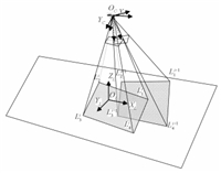
C. Rotation Around the ${x,y,z}$ AxesA case arises when the lander possesses rotational movement around the $x,y,z$ axes with the rotation angles $\psi$,$\theta$,$\phi$. Assuming the $z$ axis of the lander is vertical to the ground plane and points to the origin of the landing site cartographic coordinate system in the first frame,perspectives and projections of the four FOV corners in the second image with the rotation are shown in Fig. 7 without considering the horizontal or vertical translation. Such a sequence of rotations (rotate first about the $x$ axis,then the $y$ axis,and finally the $z$ axis) can be represented as the multiplication of three matrices,one for each axis of the coordinate system,depending on the order of rotation around the axes.
| $R = {R_z}(\phi ){R_y}(\theta ){R_x}(\psi )$ | (15) |
|
Download:
|
| Fig. 7. Rotation scenario of camera pair. | |
Using rigid body dynamics,the coordinates of the FOV corner $L^{i+1}_1$ in camera coordinate system $O_c-X_cY_cZ_c$ are
| $\left[{\begin{array}{*{20}{c}} {{x_{c_1^{i + 1}}}}\\ {{y_{c_1^{i + 1}}}}\\ {{z_{c_1^{i + 1}}}} \end{array}} \right] = C_z^i{R^{\rm{T}}}\left[{\begin{array}{*{20}{c}} {\frac{1}{{\sqrt 2 }}\tan \frac{\gamma }{2}}\\ {\frac{1}{{\sqrt 2 }}\tan \frac{\gamma }{2}}\\ 1 \end{array}} \right].$ | (16) |
Further,the coordinates of the intersection point of the FOV line $O_cL_1^{i+1}$ and the ground plane are
| $\begin{array}{l} {x_{L_1^{i + 1}}} = {C_z}\frac{{{x_{c_1^{i + 1}}}}}{{{z_{c_1^{i + 1}}}}},\\ {y_{L_1^{i + 1}}} = {C_z}\frac{{{y_{c_1^{i + 1}}}}}{{{z_{c_1^{i + 1}}}}}. \end{array}$ | (17) |
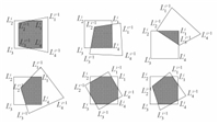
Similarly,the other coordinates limited by FOVs can be obtained. In such a scenario,it is essential to compute the overlapping area between adjacent images corresponding to their perspective quadrilaterals. Obviously,both quadrilaterals are convex,as well as the intersection polygon. The overlapping regions can be divided into many cases (some of which are shown in Fig. 8). In order to compute the overlapping area,the position of the vertexes and the quadrilateral edge intersections should be considered,and the algorithm goes as follows.
|
Download:
|
| Fig. 8. Examples of intersection polygon of two FOVs caused by rotation. | |
1) For each vertex of the first quadrilateral,check whether it is contained inside the second one. If it is,store coordinates of the point.
2) For each vertex of the second quadrilateral,check whether it is contained inside the first one. If it is,store coordinates of the point.
3) For each edge of one of the quadrilaterals (no matter which one),check intersections with edges of the other. Store coordinates of intersection points.
4) Order the triangles to form a convex polygon.
5) Compute the area using the shoelace formula[9] as a cyclic sum of determinants:
| $S = \frac{1}{2}\left| {\sum\limits_{i = 1}^n {\det } \left( {\begin{array}{*{20}{c}} {{x_i}}&{{x_{i + 1}}}\\ {{y_i}}&{{y_{i + 1}}} \end{array}} \right)} \right|,$ | (18) |
where $S$ is the area of the overlapping region,$n$ is the number of sides of the polygon,and $(x_i,y_i),~i=1,2,\cdots,n$ are the vertexes of the polygon ordered in step 4. Note that $x_{n+1}=x_1$,and $y_{n+1}=y_1$.
The algorithm can also be used for the computation of pure 3D translation and both rotation and translation. In a similar way,the overlap area among more than two successive frames can be computed.
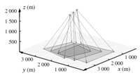
D. Motion Constraint SimulationIn this section,simulation of the Mars exploration rover (MER) descending and landing is taken[1]. The series of simulation results are carried out to reflect partially the major aim of establishing the relationship between the motion and the overlapping area. As shown in Fig. 9 three images are taken during descent at roughly 2 000 m,1 700 m and 1 400 m above the Mars surface. The 45-degree FOV navigation camera with focal length 14.67 mm is selected,because it has the best balance between pixel resolution and image overlap given the descent dynamics. It starts by tracking two features between the first image and the second,and two features between the second image and the third. The images are taken 13.75 s apart,given a nominal descent speed of 75 m/s.
|
Download:
|
| Fig. 9. Mars landing and the FOVs of lander. | |
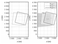
Using the overlapping area computation algorithm in Section Ⅱ,the vertexes and the quadrilateral edge intersections can be found out. The different overlap regions from frame to frame can be computed and represented in different colors as shown in Fig. 10.
|
Download:
|
| Fig. 10. Overlap regions of different images. | |
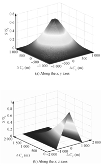
Fig. 11 (a) shows a schematic relationship between $S/S_0$ and the translation along $x$,$y$ axes from 2 000 meters to 1 700 meters,where $S$ is the overlapping area,and $S_0$ is the projected visual area in the first image. The maximum ratio of area is 85 %,because the projected visual area becomes smaller during descent. In order to maintain overlapping area ratio greater than 70 %,it needs that the horizontal velocity is at most 104 m/s when the lander descends from 2 000 m to 1 700 m,and 85 m/s is the maximum horizontal velocity when descending from 1 700 m to 1 400 m.
|
Download:
|
| Fig. 11. Relationship between S/S0 and translation. | |
Indeed,in the descending and landing process,the horizontal velocity of the lander is no more than decameters per second. According to (7),(9),(11),and (13),the overlapping area is larger if the attitude of lander is higher. If the lander takes images at high altitude,for example,at the time of the heat shield separation (about 5$\sim$9 km),the constraint of the horizontal velocity is about hundreds of m/s.
Fig. 11 (b) shows the relationship between $S/S_0$ and the translation along the $x$,$z$ axes (velocity in direction $y$ is assumed to be zero). Simulation results are presented to show that if the horizontal velocity in $x$ direction expected during descent is 30 m/s,the vertical velocity should be less than 333 m/s when the lander descends from 2 000 m to 1 700 m.
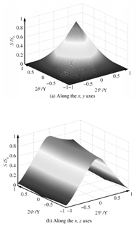
Without considering translation,formula (18) makes for a relaively easy calculation of the overlapping area. The relationship between $S/S_0$ and rotation around the $x$,$y$ axes is shown in Fig. 12 (a),in which $\psi$ ,$\theta$ are the rotation of radians about the $x$ and $y$ axes,respectively; $\gamma$ is the FOV angle. Obviously,there is no overlapping region if the rotation radians around the two axes exceed half of $\gamma$. To keep overlapping area ratio more than 70 %,the rotation angle should be less than about $5.9^{\circ}$.
|
Download:
|
| Fig. 12. Relationship between S/S0 and rotation. | |
The relationship between $S/S_0$ and rotation around the $x$,$z$ axes is shown in Fig. 12 (b),where $\phi$ is the rotation of radians about the $z$ axis. As can be seen from the graph,if the lander just rotates around the $z$ axis,the minimum overlapping area ratio is 75 %,and rotating around the $z$ axis has smaller effects on the overlapping area than rotating around the $x$ axis.
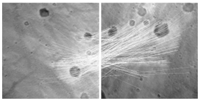
Ⅲ. HORIZONTAL VELOCITY ESTIMATION USING FEATURE MATCHING A. Feature Points Matching and Horizontal Velocity EstimationHorizontal velocity is estimated by feature points matching between two consecuive images of the sequence acquired during the descent phase. Recently,feature points matching algorithm named affine scale-invariant feature transform (ASIFT) has been proposed[14]. It simulates all possible image views and thus is fully affine invariant. ASIFT can handle much higher transition tilts than scale-invariant feature transform (SIFT)[15] or speeded up robust feature (SURF)[16],and it has characteristics of translation,scale,rotation and affine invariant. Examples of matched ASIFT features (384 points matching) are shown in Fig. 13,where MER-B landing images are taken at altitudes of approximately where and 1 690 m.
|
Download:
|
| Fig. 13. Feature points matching by ASIFT. | |
Since several hundreds of feature points can be tracked in the overlapping area of the image sequence,such correspondences are used to estimate the relative position between two views,which is the essential matrix $E$. To this purpose,we adopt an approach which exploits a prior knowledge on the attitude and altitude measurements (Fig. 14).

|
Download:
|
| Fig. 14. Comparison of feature matching by different algorithms. | |
Correspondence methods for extracting 3D structure from two views of a given scene are based on the epipolar geometry. $\{( m_i,m'_i)\}_{i=1}^n$ are the points in the scene projected to the first and the second views. The relationship between $ m_i$ and $ m'_i$ is described by the formula $ {m'}_i^{\rm T} {E{ m}}_i$,where $ m_i=[u_i$ $v_i$ $f]^{\rm T}$ and $ m'_i=[u'_i$ $v'_i$ $f$]$^{\rm T}$ include the image coordinates of the matching points and the focus. $E$ is the essential matrix,expressing cross product as matrix multiplication,
| $E = t \times R = {[t]_ \times }R,$ | (19) |
where $[{ t}]_\times=\left[\begin{array}{ccc} 0 & -t_z & t_y\\t_z & 0 &-t_x\\-t_y & t_x & 0 \end{array}\right]$,$t_x$,$t_y$ and $t_z$ denote the relative position,and $R$ is the rotation matrix between two image coordinate system.
Calculating the essential matrix requires the knowledge of the intrinsic camera plus a number of corresponding pairs of points from the two views,which have already been obtained in the earlier stage. In addition,ground relative attitude $R$ comes from inertial measurement unit (IMU),and vertical altitude $t_z$ comes from radar altimeter. So the epipolar geometry can be reconstructed by estimating the essential matrix from point correspondences. Each correspondence leads to a homogeneous equation of the simple form,i.e.,
| ${a_i}\frac{{{t_x}}}{{{t_z}}} + {b_i}\frac{{{t_y}}}{{{t_z}}} + {c_i} = 0,$ | (20) |
where
$\begin{array}{l} {a_i} = - f{R_{21}}{{u'}_i} - f{R_{22}}{{v'}_i} - {f^2}{R_{23}} + \\ \quad {R_{32}}{v_i}{{u'}_i} + {R_{32}}{v_i}v{'_i} + f{R_{33}}{v_i},\\ {b_i} = f{R_{11}}{{u'}_i} + f{R_{12}}{{v'}_i} + {f^2}{R_{13}} - \\ \quad {R_{31}}{u_i}{{u'}_i} - {R_{32}}{u_i}v{'_i} - f{R_{33}}{u_i},\\ {c_i} = - {R_{11}}_i{v_i}u{'_i} - f{R_{33}}{u_i},\\ {R_{21}}{u_i}{{u'}_i} + {R_{22}}{u_i}v{'_i} + f{R_{23}}{u_i}. \end{array}$
Two unknown parameters $t_x$,$t_y$ can be estimated using at least two corresponding point pairs. But there are normally more than dozens of matching points,so the method of least squares is used for calculating the parameters of the best fit. Thus $t_x$ and $t_y$ are easy to be computed and given by
| $\frac{1}{{{t_z}}}\left[{\begin{array}{*{20}{c}} {{t_x}}\\ {{t_y}} \end{array}} \right] = {C^{ - 1}}{A^{\rm{T}}}L,$ | (21) |
where
$A = \left[{\begin{array}{*{20}{c}} {{a_1}}&{{b_1}}\\ {{a_2}}&{{b_2}}\\ \vdots & \vdots \\ {{a_i}}&{{b_i}}\\ \vdots & \vdots \\ {{a_n}}&{{b_n}} \end{array}} \right],C = {A^{\rm{T}}}A,L = - \left[{\begin{array}{*{20}{c}} {{c_1}}\\ {{c_2}}\\ \vdots \\ {{c_i}}\\ \vdots \\ {{c_n}} \end{array}} \right].$
After estimating the relative position,the horizontal velocity can be easily gained by the image interval time and the rotation matrix. In addition,errors in the attitude and altitude estimates,and radial distortion would leak into the horizontal velocity estimate. This coupling of sensor errors have to be accounted for when generating a total velocity estimation error budget for simulation. Some of the representative parameters are shown in Table Ⅰ.
|
|
Table Ⅰ REPRESENTATIVE PARAMETERS IN SIMULATION |
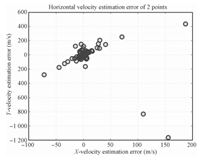
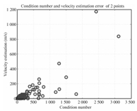
Obviously,the estimation of horizontal velocity is critically important,with any miscalculation potentially leading to the mission$'$s failure. But in the computation of $t_x$ and $t_y$,the least squares may not be the ideal solution when gross errors appear (up to hundreds of m/s,see Fig. 15),especially using less than 5 equations. The gross errors are not caused by the egregious mismatches,but due to the ill-conditioned matrices with large condition number $\kappa(A)=\|A\|\|A^{-1}\|$ (Fig. 16). The condition number times the relative change in the data bound the relative change in the solution. The proof is as follows.
|
Download:
|
| Fig. 15. Velocity estimation with gross error. | |
|
Download:
|
| Fig. 16. Velocity estimation error and the condition numbers. | |
{\bf Proof.} Let $x$ denote the solution vector of the linear system $A{ x}= b$. If we change $ b$ to $ b+\Delta b$,the new solution is $ x+\Delta x$ with
| $A(x + \Delta x) = b + \Delta b.$ | (22) |
The change in $ x$ is
| $\Delta x = {A^{ - 1}}\Delta b.$ | (23) |
By using the property of matrix norm,we obtain that
| $\left\| {\Delta x} \right\| \le \left\| {{A^{ - 1}}} \right\| \cdot \left\| {\Delta b} \right\|,$ | (24) |
and
| $\left\| A \right\| \cdot \left\| x \right\| \ge \left\| b \right\|.$ | (25) |
Dividing (24) by (25),we have
| $\frac{{\left\| {\Delta x} \right\|}}{{\left\| x \right\|}} \le \left\| A \right\| \cdot \left\| {{A^{ - 1}}} \right\| \cdot \frac{{\left\| {\Delta b} \right\|}}{{\left\| b \right\|}} = \kappa (A) \cdot \frac{{\left\| {\Delta b} \right\|}}{{\left\| b \right\|}}.$ | (26) |
If a small change is made in the coefficient matrix $A$ while keeping vector $ b$ fixed,then
| $\frac{{\left\| {\Delta x} \right\|}}{{\left\| {x + \Delta x} \right\|}} \le \kappa (A) \cdot \frac{{\left\| {\Delta A} \right\|}}{{\left\| A \right\|}}.$ | (27) |
So matrix $C=A^{\rm T}A$ is badly conditioned or ill-conditioned if condition number $\kappa(A)=\|A\|\|A^{-1}\|$ is large,the relative error in $ x$ can be much larger than that in $ b$ or $A$.
Therefore it is extremely important in the work of numerical modeling to ensure that the constructed matrix has a low condition number. Existing methods for this problem are mostly based upon the singular value decomposition (SVD) methods,iterative methods[17],or some other methods[18, 19]. These methods have been proven to be a cure for such ill-conditioned linear algebraic systems,although they generally converge very slowly or do not have very obvious effects on some ill-conditioned matrices.
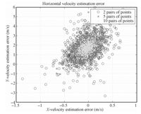
The matrices of ill-conditioned systems are characterized by large condition numbers,and usually dozens of matching points are available. Then the points that associate with large condition number matrices (using matrix $A$ instead of matrix $C$ for the sake of simplicity) can be firstly eliminated before solving final governing equations. By this way,complex calculations mentioned above can be avoided. Furthermore,the solution becomes more stable. Thousands of Monte Carlo runs have been conducted using this algorithm to produce horizontal velocity estimation,and no gross errors appear. Results are presented in Fig. 17.
|
Download:
|
| Fig. 17. Velocity estimation error after elimination of large condition numbers. | |
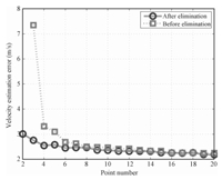
Fig. 18 shows an obvious improvement in accuracy,after eliminating the large condition number matrices ($\kappa(A)>10$). The velocity estimating accuracy increases with the number of the available feature points,both in matrices with or without elimination of large condition numbers. Addressing the least square theory,the accuracy of estimating parameters for linear system embedded in noise is inversely proportional to $\sqrt{n-t}$,where $n$ is the number of equations and $t$ is the number of parameters. Using 6 pairs of points,the error of velocity estimation can reach as low as 2.5 m/s,and little increase in accuracy is achieved with more than 10 feature points. There is also an increase of systematic errors (about 2 m/s in this simulation) tending to be consistent in the radial lens distortion variation and the direction of lander movement. When metric and quality results are required,automatically correcting the radial lens distortion is necessary before computing the velocity.
|
Download:
|
| Fig. 18. Relationship between velocity estimation error and point number. | |
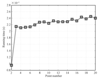
The estimation accuracy increases at the expense of long computation time. In principle,for the least squares with $n$ equations and $t$ unknown parameters,it takes ${\rm O}(t^2n)$ to multiply $A^{\rm T}$ by $A$,${\rm O}(tn)$ to multiply $A^{\rm T}$ by $L$,${\rm O}(t^3)$ to compute the Cholesky or LU factorization of $A^{\rm T}A$ and then to compute the product $C^{-1} A^{\rm T} L$. Asymptotically,${\rm O}(t^2n)$ dominates ${\rm O}(tn)$,so the ${\rm O}(tn)$ can be ignored. Since $n\geq t$,which means that ${\rm O}(t^2n)$ asymptotically dominates ${\rm O}(t^3)$,the total time complexity is ${\rm O}(t^2n)$. Particularly,computing the Cholesky or LU decomposition of $A^{\rm T}A$ takes significantly longer than multiplying $ A^{\rm T}$ by $A$. The relationship between running time and the number of points is shown in Fig. 19.
|
Download:
|
| Fig. 19. Relationship between running time and point number. | |
When $n=2$,the running time is significantly reduced,because it does not need to compute the inverse matrix with decomposition.
Ⅳ. CONCLUSIONIn this paper,a new concept for visual navigation is presented based on the analysis of motion constraints and stable estimation of horizontal velocity is determined as well. Based on the projection of FOV lines,a method is presented to calculate the overlapping area between the consecuive frames. The percentage of overlapping specifies the allowable range of movement including translation and rotation for constraints. The proposed approach in this paper uses more than two feature points to estimate the horizontal velocity,which is more accurate than the method of DIMES,where only two points are used. Further,the proposed approach in this paper is able to eliminate the large condition number matrices to improve its stability.
| [1] | Johnson A, Willson R, Goguen J, Alexander J, Meller D. Field testing of the mars exploration rovers decent image motion estimation system. In:Proceedings of the 2005 International Conference Robotics and Automation. Barcelona, Spain:IEEE, 2005. 4463-4469 |
| [2] | Tweddle B E. Computer Vision Based Navigation for Spacecraft Proximity Operations[Master dissertation], Massachusetts Institute of Technology, USA, 2010. |
| [3] | van Pham Bach V P, Lacroix Simon L, Devy Michel D. Vision-based absolute navigation for descent and landing. Journal of Field Robotics, 2012, 29(4):627-647 |
| [4] | Cheng Y, Goguen J, Johnson A, Legetr C, Matthies L, Martin M S, Willson Ret al. The Mars exploration rovers descent image motion estimation system. In:Proceedings of the 2004 IEEE Intelligent Tutoring Systems, Los Alamitos, USA:IEEE, 2004. 13-21 |
| [5] | Johnson A, Willson R, Cheng Y, Goguen J, Leger C, Sanmartin M, Matthies Let al. Design through operation of an image-based velocity estimation system for Mars landing. International Journal of Computer Vision, 2007, 74(3):319-341 |
| [6] | Harris C, Stevens M. A combined corner and edge detector. In:Proceedings of the 4th Alvey Vision Conference. England:University of Manchester, 1988. 147-151 |
| [7] | Flandin G, Polle B, Frapard B, Vidal P, Philippe C, Voirin T. Vision based navigation for planetary exploration. In:Proceedings of the 32nd Annual AAS Rocky Mountain Guidance and Control Conference. Breckenridge, Colorado:2009. 277-296 |
| [8] | Lanza Piergiorgio L, Noceti Nicoletta N, Maddaleno Corrado M, Toma Antonio T, Zini Luca Z, Odone Francesca O. A vision-based navigation facility for planetary entry descent landing. In:Proceedings of the 12th International Conference on Computer Vision. Florence, Italy:Springer, 2012. 546-555 |
| [9] | Rigatos Gerasimos G R. Nonlinear Kalman filters and particle filters for integrated navigation of unmanned aerial vehicles. Robotics and Autonomous Systems, 2012, 60(7):978-995 |
| [10] | Li M Y, Mourikis Anastasion I M. High-precision, consistent EKF-based visual-inertial odometery. International Journal of Robotics Research, 2013, 32(6):690-711 |
| [11] | Paul A J, Lorraine E P. A historical compilation of software metrics with applicability to NASA's Orion spacecraft flight software sizing. Innovations in Systems and Software Engineering, 2011, 7(3):161-170 |
| [12] | Dubois M O, Parkes S, Dunstam M. Testing and validation of planetary vision-based navigation systems with PANGU. In:Proceedings of the 21st International Symposium on Space Flight Dynamics. Toulouse, France:ISSFD, 2009 |
| [13] | Newcombe R A, Davison A J. Live dense reconstruction with a single moving camera. In:Proceedings of the 2010 International Conference on Computer Vision and Pattern Recognition. San Francisco, USA:IEEE, 2010. 1498-1505 |
| [14] | Morel J M, Yu G S. ASIFT:a new framework for fully affine invariant image comparison. SIAM Journal on Imaging Sciences, 2009, 2(2):438-469 |
| [15] | Lowe D G. Distinctive image features from scale-invariant keypoints. International Journal of Computer Vision, 2004, 60(42):91-110 |
| [16] | Bay H, Ess A, Tuytelaars T, van Gool L V. SURF:speeded up robust features. Computer Vision and Image Understanding, 2008, 110(3):346-359 |
| [17] | Peris R, Marquina A, Candela V. The convergence of the perturbed Newton method and its application for ill-conditioned problems. Applied Mathematics and Computation, 2011, 218(7):2988-3001 |
| [18] | Salahi M. On regularization of ill-conditioned linear systems. Journal of Applied Mathematics, 2008, 5(17):43-49 |
| [19] | Brezinski C, Novati P, Redivo Z M. A rational Arnoldi approach for ill-conditioned linear systems. Journal of Computational and Applied Mathematics, 2012, 236(8):2063-2077 |
 2015, Vol.2


