2. the Key Lab of System and Control, Academy of Mathematics and System Science,Chinese Academy of Sciences, Beijing 100190, China
PERMANENT magnet synchronous motors (PMSMs) have been widely used in the motion control field,transmission control field,servo system and so on,thanks to theirs features of small volume,high power,low noise and high torque-to-current ratio. Compared with other motors,the PMSMs have many advantages,but theirs mathematical model has the characteristics of high order,nonlinear,strong coupling and multi-variables. Therefore,it is difficult to design theirs controller. Because the PMSMs has an irreplaceable role in engineering application,huge economic benefit will be achieved and good motion/traction performance will be obtained if it has been well controlled. An increasing number of scholars came up with all kind of control strategies in this field in recent decades of years. For example,in order to deal with the disturbance of parameter and load torque,robust control[1, 2] was developed. Adaptive control[3, 4] has been researched so that the controller can adapt to the change of parameter and/or load. In [5, 6],some performance indexes were optimized when predictive control was used. In order to get good output performance even the motor's parameters change with time,model reference adaptive control[7] was introduced in this field. Sensorless controller[8] and observerbased[9] controller were designed to reduce the cost of controller and minimize the volume of controller. Fuzzy controller[10, 11] was widely used to handle the structured and unstructured uncertainty. In order to deal with the disturbances,slide mode controller[12] has been researched. Internal model control was utilized to improve the robustness of the whole system[13]. In [14],torque feedforward controller was established to achieve good dynamic performance. Besides,many other control strategies were developed,such as near optimal control[15] and neural network control[16]. Recently,hybrid control methods[10, 13] have been widely adopted.
Interval matrix is often used to cope with systems' parameters are unknown but vary (or locate) in a certain range[17, 18]. Its mainly idea is an interval matrix whose elements change (or locate) in a specific range can be expressed by several matrices which can be further handled by other methods. For a given PMSM,restricted by supply power,operation environment,protection equipment and so on, current and speed are and must be in a specific range likes rated range. Therefore,interval matrix can be introduced to design the controller of PMSMs. Besides,although many control strategies have been developed,in fact,PI control method is still a main control strategy in engineering application because it is easy to implement and has a good control performance,i.e.,many advance control strategies have not been widely adopted in engineering because it is not easy to apply or its cost is higher than that of the conventional PI control method. In order to get a easy realized controller which can deal with load uncertainty,in this paper, robust controllers are developed via interval matrix and PI control idea.
This paper is organized as follows. In Section Ⅲ,the mathematical model of PMSMs and lemmas are presented. Robust control strategies are developed in Section Ⅲ. To verify the effectiveness of the proposed methods,in section Ⅳ,simulations are carried out via Matlab/Simulink soft. In Section V,some conclusions are obtained.
Ⅲ. MODEL DESCRIPTION AND LEMMASAccording to [19, 20],the mathematical model of PMSMs can be expressed as
| $\frac{{{\rm{d}}{i_d}}}{{{\rm{d}}t}} = - \frac{{{R_s}}}{{{L_{sd}}}}{i_d} + \frac{{{L_{sq}}}}{{{L_{sd}}}}\omega {i_q} + \frac{1}{{{L_{sd}}}}{u_d},$ $\frac{{{\rm{d}}{i_q}}}{{{\rm{d}}t}} = - \frac{{{L_{sd}}}}{{{L_{sq}}}}\omega {i_d} - \frac{{{R_s}}}{{{L_{sq}}}}{i_q} - \frac{1}{{{L_{sq}}}}\omega {\psi _r} + \frac{1}{{{L_{sq}}}}{u_q},$ $\frac{{{\rm{d}}\omega }}{{{\rm{d}}t}} = \frac{{n_p^2}}{J}({L_{sd}} - {L_{sq}}){i_d}{i_q} + \frac{{n_p^2}}{J}{\psi _r}{i_q} - \frac{{{n_p}}}{J}{T_l} - \frac{{{B_f}}}{J}\omega ,$ | (1) |
where ${L_{sd}}$,${L_{sq}}$ are $d{\rm{ - }}$ and $q$-axis inductance; ${R_s}$ is stator resistances; ${\psi _r}$ is permanent magnet flux linkage; ${n_p}$ is the number of pole pairs; ${B_f}$ is frictional coefficient; $J$ is moment inertia; ${i_d}$ and ${i_q}$ are $d{\rm{ - }}$ and $q$-axis stator currents; $\omega $ is rotor angular velocity; ${u_d}$ and ${u_q}$ are $d{\rm{ - }}$ and $q$-axis voltages and ${T_l}$ is load torque.
Usually,the model expressed as (1) could not accurately describe the actual model of PMSMs because of the existence of disturbance. For example,resistance will increase with the rise of temperature. In other words,disturbances must be considered in the model to make the model more accurately present the actual model. Thus,the following model is established if disturbances are considered.
| $\begin{array}{l} \frac{{{\rm{d}}{i_d}}}{{{\rm{d}}t}} = - \frac{{{R_s}}}{{{L_{sd}}}}{i_d} + \frac{{{L_{sq}}}}{{{L_{sd}}}}\omega {i_q} + \frac{1}{{{L_{sd}}}}{u_d} + {d_d},\\ \frac{{{\rm{d}}{i_q}}}{{{\rm{d}}t}} = - \frac{{{L_{sd}}}}{{{L_{sq}}}}\omega {i_d} - \frac{{{R_s}}}{{{L_{sq}}}}{i_q} - \frac{1}{{{L_{sq}}}}\omega {\psi _r} + \frac{1}{{{L_{sq}}}}{u_q} + {d_q},\\ \frac{{{\rm{d}}\omega }}{{{\rm{d}}t}} = \frac{{n_p^2}}{J}({L_{sd}} - {L_{sq}}){i_d}{i_q} + \frac{{n_p^2}}{J}{\psi _r}{i_q} - \frac{{{n_p}}}{J}{T_l} - \frac{{{B_f}}}{J}\omega + {d_\omega }, \end{array}$ | (2) |
where ${d_d}$,${d_q}$ and ${d_\omega }$ represent the total disturbances acting on $d$-axis,$q$-axis and motion equations, respectively,which may be caused by the environment or the change of parameter. And in fact,the disturbances and the load change very slowly,i.e.,the following equations usually are satisfied.
| $\frac{{{\rm{d}}{d_d}}}{{{\rm{d}}t}} \approx 0,\frac{{{\rm{d}}{d_q}}}{{{\rm{d}}t}} \approx 0,\frac{{{\rm{d}}{d_\omega }}}{{{\rm{d}}t}} \approx 0,\frac{{{\rm{d}}{T_l}}}{{{\rm{d}}t}} \approx 0.$ | (3) |
Lemma 1[21]. For any scalar $\varepsilon > 0$,$X$ and $Y$ are real matrices with appropriate dimensions so that the following inequality is obtained.
$${X^{\rm{T}}}Y + {Y^{\rm{T}}}X \le \frac{1}{\varepsilon }{X^{\rm{T}}}X + \varepsilon {Y^{\rm{T}}}Y.$$Lemma 2[22]. Given symmetric matrix
$$S(x) = \left( {\begin{array}{*{20}{c}} {{S_{11}}(x)}&{{S_{12}}(x)}\\ {S_{12}^{\rm{T}}(x)}&{{S_{22}}(x)} \end{array}} \right)$$and ${S_{11}}(x) \in {{\bf{R}}^{K \times K}}$,the following conditions are equivalent:
1) $S(x) < 0$;
2) ${S_{11}}(x) < 0,{S_{22}}(x) - S_{12}^{\rm{T}}(x)S_{11}^{ - 1}(x){S_{12}}(x) < 0$;
3) ${S_{22}}(x) < 0,{S_{11}}(x) - {S_{12}}(x)S_{22}^{ - 1}(x)S_{12}^{\rm{T}}(x) < 0.$
If matrices ${A^m} = {\rm{ }}{[a_{ij}^m]_{n \times n}}$ and ${A^M} = {[a_{ij}^M]_{n \times n}}$ satisfy $a_{ij}^m \le a_{ij}^M$ for all $1 \le i,j \le n$,$\left[{\begin{array}{*{20}{c}} {{A^m}}&{{A^M}} \end{array}} \right] = \{ [{a_{ij}}]:a_{ij}^m \le {a_{ij}} \le a_{ij}^M,i \le i,j \le n\} $ is established. Assume $A \in {\rm{ }}{{\bf{R}}^{n \times n}}$ and $A \in [\begin{array}{*{20}{c}} {{A^m}}&{{A^M}} \end{array}]$ ,then $A$ is called interval matrix.
Lemma 3[17]. For a given interval matrices $A \in \left[ {\begin{array}{*{20}{c}} {{A^m}}&{{A^M}} \end{array}} \right]$ and $A \in {{\bf{R}}^{n \times n}}$,$A$ can be rewritten as follows.
$$A = {A_0} + E\Delta G,\Delta \in {\Delta ^*},$$where ${A_0} = \frac{1}{2}({A^M} + {A^m})$,$H = {[{h_{ij}}]_{n \times n}} = \frac{1}{2}({A^M} - {A^m})$. Elements of matrix ${A^m},{A^M}$ are made up of the low bound and the upper bound of the elements in matrix $A$,respectively. Obviously,each element of matrix $H$ is nonnegative.
$$\begin{array}{l} {\Delta ^*} = \{ \Delta \in {{\bf{R}}^{{n^2} \times {n^2}}}|\Delta = \\ {\rm{diag}}\left\{ {\begin{array}{*{20}{c}} {{\chi _{11}}}& \cdots &{{\chi _{1n}}}& \cdots &{{\chi _{n1}}}& \cdots &{{\chi _{nn}}} \end{array}} \right\}\\ |{\chi _{ij}}| \le 1,i,j = 1, \cdots ,n\} ,\\ E = \left[ {\begin{array}{*{20}{c}} {\sqrt {{h_{11}}} {e_1}}& \cdots &{\sqrt {{h_{1n}}} {e_1}}& \cdots \end{array}\begin{array}{*{20}{c}} {\sqrt {{h_{n1}}} {e_n}}& \cdots &{\sqrt {{h_{nn}}} {e_n},} \end{array}} \right]\\ G = \left[ {\begin{array}{*{20}{c}} {\sqrt {{h_{11}}} {e_1}}& \cdots &{\sqrt {{h_{1n}}} {e_n}}& \cdots \end{array}\begin{array}{*{20}{c}} {\sqrt {{h_{n1}}} {e_1}}& \cdots &{\sqrt {{h_{nn}}} {e_n}} \end{array}} \right]_{n \times {n^2}}^{\rm{T}}. \end{array}$$Lemma 4[23]. For any given interval matrix $A \in [\begin{array}{*{20}{c}} {{A^m}}&{{A^M}} \end{array}]$,matrix ${A_0} = \frac{1}{2}({A^M} + {A^m})$ and $H = {[{h_{ij}}]_{n \times n}} = \frac{1}{2}({A^M} - {A^m})$,$A$ can be represented as $A = {A_0} + \sum\nolimits_{i,j = 1}^n {{e_i}{f_{ij}}e_j^{\rm{T}}} $,$\left| {{f_{ij}}} \right| \le {\rm{ }}{h_{ij}}.$
Notations. $I$ is identity matrix with appropriate dimension and ${e_i}$ is the $ith$ column of unit matrix with appropriate dimension. $X < Y$,where $X$ and $Y$ are symmetric matrices,means that the matrix $Y - X$ is positive definite.
Ⅲ. Robust controlAlthough many advance control strategies have been developed in the PMSMs control field,PI controller is still currently main control strategy in practical application because it is easy to implement and can get good control performance. Therefore,in this section,robust controllers of PMSMs will be developed via PI control idea.
A. ROBUST CONTROLLERAccording to the character of PMSMs,the state variables and control inputs can be chosen as
| $\begin{array}{l} X = {\left[{\begin{array}{*{20}{c}} {{i_d}}&{\frac{{d{i_d}}}{{dt}}}&{\frac{{d{i_q}}}{{dt}}}&{\omega - {\omega ^*}}&{\frac{{d(\omega - {\omega ^*})}}{{dt}}} \end{array}} \right]^{\rm{T}}},\\ U = {\left[{\begin{array}{*{20}{c}} {{u_d}}&{{u_q}} \end{array}} \right]^{\rm{T}}}, \end{array}$ | (4) |
where ${\omega ^*}$ is the desired speed of the system,and is a constant.
According to (2)~(4),the following state equation is obtained.
| $\dot X = A(t)X + B\dot U,$ | (5) |
where
$$A(t){\rm{ }} = {\left[{{a_{ij}}} \right]_{5 \times 5}} = \left[{\begin{array}{*{20}{c}} 0&1\\ 0&{ - \frac{{{R_s}}}{{{L_{sd}}}}}\\ 0&{ - \frac{{{L_{sd}}}}{{{L_{sq}}}}\omega }\\ 0&0\\ 0&{\frac{{n_p^2}}{J}({L_{sd}} - {L_{sq}}){i_q}} \end{array}} \right.\left. {\begin{array}{*{20}{c}} 0&0&0\\ { - \frac{{{L_{sq}}}}{{{L_{sd}}}}\omega }&0&{\frac{{{L_{sq}}}}{{{L_{sd}}}}{i_q}}\\ { - \frac{{{R_s}}}{{{L_{sq}}}}}&0&{ - (\frac{{{L_{sd}}}}{{{L_{sq}}}}{i_d} + \frac{{{\psi _r}}}{{{L_{sq}}}})}\\ 0&0&1\\ {\frac{{n_p^2}}{J}(({L_{sd}} - {L_{sq}}){i_d} + {\psi _r})}&0&{ - \frac{B}{J}} \end{array}} \right],$$ $$B{\rm{ }} = {\left[{\begin{array}{*{20}{c}} 0&{\frac{1}{{{L_{sd}}}}}&0&0&0\\ 0&0&{\frac{1}{{{L_{sq}}}}}&0&0 \end{array}} \right]^{\rm{T}}}.$$For a given PMSM which is constrained by the voltage source, switch frequency,protect facilities,operating environment and so on,current and speed are and must be in a certain range,such as rated range. In other words,current is not larger than rated current and speed is not higher than rated speed. Hence,the following assumptions are reasonable.
| $i_d^m \le {i_d} \le i_d^M,i_q^m \le {i_q} \le i_q^M,{\omega ^m} \le \omega \le {\omega ^M},$ | (6) |
where $i_d^m,i_d^M,i_q^m,i_q^M,{\omega ^m}$and ${\omega ^M}$ are the lower bound and the upper bound of ${i_d},{i_q}$ and $\omega $,respectively.
Based on condition (6),$A(t)$ is viewed as interval matrix,and according to Lemma 3,$A(t)$ can be rewritten as
| $A(t) = {A_0} + E\Delta (t)M,\Delta (t) \in {\Delta ^*},$ | (7) |
where
$$\begin{array}{l} {A_{c0}} = \left[ {\begin{array}{*{20}{c}} 0&1&0&0&0\\ 0&{ - \frac{{{R_s}}}{{{L_{sd}}}}}&{a_{23}^{c0}}&0&{a_{25}^{c0}}\\ 0&{a_{32}^{c0}}&{ - \frac{{{R_s}}}{{{L_{sq}}}}}&0&{a_{35}^{c0}}\\ 0&0&0&0&1\\ 0&{a_{52}^{c0}}&{a_{53}^{c0}}&0&{ - \frac{B}{J}} \end{array}} \right],\\ a_{23}^{c0} = - \frac{{{L_{sq}}({\omega ^M} + {\omega ^m})}}{{2{L_{sd}}}},a_{25}^{c0} = \frac{{{L_{sq}}}}{{2{L_{sd}}}}(i_q^M + i_q^m),\\ a_{32}^{c0} = - \frac{{{L_{sd}}({\omega ^M} + {\omega ^m})}}{{2{L_{sq}}}},a_{35}^{c0} = - \left( {\frac{{{L_{sd}}(i_d^M + i_d^m)}}{{2{L_{sq}}}} + \frac{{{\psi _r}}}{{{L_{sq}}}}} \right),\\ a_{52}^{c0} = \frac{{n_p^2}}{{2J}}({L_{sd}} - {L_{sq}})(i_q^M + i_q^m),\\ a_{53}^{c0} = \frac{{n_p^2}}{J}\left( {({L_{sd}} - {L_{sq}})\frac{{(i_d^M + i_d^m)}}{2} + {\psi _r}} \right),\\ \begin{array}{*{20}{l}} {H = {{\left[ {{h_{ij}}} \right]}_{5 \times 5}} = \left[ {\begin{array}{*{20}{c}} 0&0\\ 0&0\\ 0&{\frac{{{L_{sd}}({\omega ^M} - {\omega ^m})}}{{2{L_{sq}}}}}\\ 0&0\\ 0&{\frac{{n_p^2}}{{2J}}|{L_{sd}} - {L_{sq}}|(i_q^M - i_q^m)} \end{array}} \right.}\\ {\left. {\begin{array}{*{20}{c}} 0&0&0\\ {\frac{{{L_{sq}}({\omega ^M} - {\omega ^m})}}{{2{L_{sd}}}}}&0&{\frac{{{L_{sq}}}}{{2{L_{sd}}}}(i_q^M - i_q^m)}\\ 0&0&{\frac{{{L_{sd}}(i_d^M - i_d^m)}}{{2{L_{sq}}}}}\\ 0&0&0\\ {\frac{{n_p^2}}{{2J}}|{L_{sd}} - {L_{sq}}|(i_d^M - i_d^m)}&0&0 \end{array}} \right],} \end{array} \end{array}$$The following theorem can be obtained.
Theorem 1. The PMSMs presented as (2) can be stabilized and the rotor angular speed can track the desired speed under the conditions (3) and (6) if there exist a symmetric and positive-definite matrix ${P_1} \in {\rm{ }}{{\bf{R}}^{5 \times 5}}$, matrix $K \in {\rm{ }}{{\bf{R}}^{2 \times 5}}$ and positive scalar $\varepsilon $ such that the following BMI holds:
| $\left[{\begin{array}{*{20}{c}} {\begin{array}{*{20}{l}} {A_0^{\rm{T}}{P_1} + {P_1}{A_0} + {K^{\rm{T}}}{B^{\rm{T}}}{P_1} + }\\ {{P_1}BK + \varepsilon {M^{\rm{T}}}M} \end{array}}&{{P_1}E}\\ {{E^{\rm{T}}}{P_1}}&{ - \varepsilon I} \end{array}} \right] < 0,$ | (8) |
And the robust control law is $\dot U = KX.$
Proof. The control law is designed as
| $\dot U = KX.$ | (9) |
Choose Lyapunov function as follows.
| ${V_1} = {X^{\rm{T}}}{P_1}X.$ | (10) |
Taking the derivative of Lyapunov function (10) with respect to $t$ along system (5) with (7) yields
| ${\dot V_1} = {X^{\rm{T}}}(A_0^{\rm{T}}{P_1} + {P_1}{A_0} + {K^{\rm{T}}}{B^{\rm{T}}}{P_1} + {P_1}BK)X + {X^{\rm{T}}}{M^{\rm{T}}}{\Delta ^{\rm{T}}}(t){E^{\rm{T}}}{P_1}X + {X^{\rm{T}}}{P_1}E\Delta (t)MX.$ | (11) |
Equation (11) can be written as follows via Lemma 1 and $\Delta {({\rm{t}})^{\rm{T}}}\Delta ({\rm{t}}) \le I$
| ${\dot V_1} \le {X^{\rm{T}}}{Q_1}X,$ | (12) |
where ${Q_1} = A_0^{\rm{T}}{P_1} + {P_1}{A_0} + {K^{\rm{T}}}{B^{\rm{T}}}{P_1} + {P_1}BK + \varepsilon {M^{\rm{T}}}M + {\rm{ }}\frac{{{P_1}E{E^{\rm{T}}}{P_1}}}{\varepsilon }.$
If ${Q_1} < 0$,the time derivative of Lyapunov function ${V_{\rm{1}}}$ is negative,which means the system can be stabilized by the controller and the PMSMs' speed can follow the desired speed according to Lyapunov stability theory. And ${Q_1} < 0$ can be expressed as (8) by Lemma 2.
There are six interval variable in matrix $A(t)$,i.e., ${a_{{\rm{23}}}}{\rm{,}}{a_{{\rm{25}}}}{\rm{,}}{a_{{\rm{32}}}}{\rm{,}}{a_{{\rm{35}}}}{\rm{,}}{a_{{\rm{52}}}}$ and ${a_{53}}$. The matrix $A(t)$ can be rewritten as follows via Lemma 4 to reduce the conservative of BMI.
| ${A_c}(t) = {A_{c0}} + {e_2}f_{23}^ce_3^{\rm{T}} + {e_2}f_{25}^ce_5^{\rm{T}} + {e_3}f_{32}^ce_2^{\rm{T}} + {e_3}f_{35}^ce_5^{\rm{T}} + {e_5}f_{52}^ce_2^{\rm{T}} + {e_5}f_{53}^ce_3^{\rm{T}},$ | (13) |
where,$|{f_{23}}| \le {h_{23}},|{f_{25}}| \le {h_{25}},|{f_{32}}| \le {h_{32}},|{f_{35}}| \le {h_{35}},|{f_{52}}| \le {h_{52}}and|{f_{53}}| \le {h_{53}}.$
The following theorem can be obtained.
Theorem 2. The PMSMs presented as (2) can be stabilized and the rotor angular speed can track the desired speed under the conditions (3) and (6) if there exist symmetric and positive-definite matrix ${P_2} \in {\rm{ }}{{\bf{R}}^{5 \times 5}}$, matrix $K \in {\rm{ }}{{\bf{R}}^{2 \times 5}}$,real scalar ${\varepsilon _{23}} > 0,{\varepsilon _{25}} > 0,{\varepsilon _{32}} > 0,{\varepsilon _{35}} > 0,{\varepsilon _{52}} > 0$ and ${\varepsilon _{53}} > 0$ > 0 such that the following BMI holds:
| $\left[{\begin{array}{*{20}{c}} {\begin{array}{*{20}{l}} {A_0^T{P_2} + {P_{c2}}{A_0} + {K^T}{B^T}{P_2} + }\\ {{P_2}BK + {\Xi _1}} \end{array}}&{{\Xi _{c2}}}\\ {\Xi _2^T}&{ - {\Xi _3}} \end{array}} \right] < 0,$ | (14) |
where
$${\Xi _1}{\rm{ }} = {\varepsilon _{23}}{({h_{23}})^2}{e_3}e_3^{\rm{T}} + {\varepsilon _{25}}{({h_{25}})^2}{e_5}e_5^{\rm{T}} + {\varepsilon _{32}}{({h_{32}})^2}{e_2}e_2^{\rm{T}} + {\varepsilon _{35}}{({h_{35}})^2}{e_5}e_5^{\rm{T}} + {\varepsilon _{52}}{({h_{52}})^2}{e_2}e_2^{\rm{T}} + {\varepsilon _{53}}{({h_{53}})^2}{e_3}e_3^{\rm{T}}$$, $$\begin{array}{l} {\Xi _2} = \left[ {\begin{array}{*{20}{c}} {{P_{c2}}{e_2}}&{{P_{c2}}{e_2}}&{{P_{c2}}{e_3}}&{{P_{c2}}{e_3}}&{{P_{c2}}{e_5}}&{{P_{c2}}{e_5}} \end{array}} \right],\\ {\Xi _3} = {\rm{diag}}\left\{ {\begin{array}{*{20}{c}} {{\varepsilon _{23}}}&{{\varepsilon _{25}}}&{{\varepsilon _{32}}}&{{\varepsilon _{35}}}&{{\varepsilon _{52}}}&{{\varepsilon _{53}}} \end{array}} \right\}, \end{array}$$and the robust control law is $\dot U = KX.$
Proof. Lyapunov function is designed as
| ${V_2} = {X^{\rm{T}}}{P_2}X.$ | (15) |
Taking the derivative of Lyapunov function (15) with respect to $t$ along system (5) with (13) yields
| $\begin{array}{l} {{\dot V}_2} = {X^{\rm{T}}}(A_0^{\rm{T}}{P_2} + {P_2}{A_0} + {K^{\rm{T}}}{B^{\rm{T}}}{P_2} + {P_2}BK)X + \qquad \\ {X^{\rm{T}}}({e_2}{f_{23}}e_3^{\rm{T}} + {e_2}{f_{25}}e_5^{\rm{T}} + {e_3}{f_{32}}e_2^{\rm{T}} + {e_3}{f_{35}}e_5^{\rm{T}} + \\ {e_5}{f_{52}}e_2^{\rm{T}} + {e_5}{f_{53}}e_3^{\rm{T}}{)^{\rm{T}}}{P_2}X + {X^{\rm{T}}}{P_2}({e_2}{f_{23}}e_3^{\rm{T}} + \\ {e_2}{f_{25}}e_5^{\rm{T}} + {e_3}{f_{32}}e_2^{\rm{T}} + {e_3}{f_{35}}e_5^{\rm{T}} + {e_5}{f_{52}}e_2^{\rm{T}} + {e_5}{f_{53}}e_3^{\rm{T}})X. \end{array}$ | (16) |
According to Lemma 1 and ${f_{ij}}^{\rm{T}}{f_{ij}} \le {({h_{ij}})^2}$,the following inequality can be obtained.
| ${V_2} \le {X^{\rm{T}}}{Q_2}X.$ | (17) |
where
$$\begin{array}{l} {Q_2} = A_0^{\rm{T}}{P_2} + {P_2}{A_0} + {K^{\rm{T}}}{B^{\rm{T}}}{P_2} + {P_2}BK + \frac{{{P_2}{e_2}e_2^{\rm{T}}{P_2}}}{{{\varepsilon _{23}}}} + \\ {\varepsilon _{23}}{({h_{23}})^2}{e_3}e_3^{\rm{T}} + \frac{{{P_2}{e_2}e_2^{\rm{T}}{P_2}}}{{{\varepsilon _{25}}}} + {\varepsilon _{25}}{({h_{25}})^2}{e_5}e_5^{\rm{T}} + \\ \frac{{{P_2}{e_3}e_3^{\rm{T}}{P_2}}}{{{\varepsilon _{32}}}} + {\varepsilon _{32}}{({h_{32}})^2}{e_2}e_2^{\rm{T}} + \frac{{{P_2}{e_3}e_3^{\rm{T}}{P_2}}}{{{\varepsilon _{35}}}} + \\ {\varepsilon _{35}}{({h_{35}})^2}{e_5}e_5^{\rm{T}} + \frac{{{P_2}{e_5}e_5^{\rm{T}}{P_2}}}{{{\varepsilon _{52}}}} + {\varepsilon _{52}}{({h_{52}})^2}{e_2}e_2^{\rm{T}} + \\ \frac{{{P_2}{e_5}e_5^{\rm{T}}{P_2}}}{{{\varepsilon _{53}}}} + {\varepsilon _{53}}{({h_{53}})^2}{e_3}e_3^{\rm{T}}. \end{array}$$If the inequality ${Q_2} < 0$ holds,it stands the time derivative of Lyapunov function ${V_{\rm{2}}}$ is negative,which means the system can be stabilized by the controller and the PMSMs' speed can follow the set point according to Lyapunov stability theory. ${Q_2} < 0$ can be written as (14) via Lemma 2.
B. Robust Controller with Feedforward CompensationIn order to further reduce the conservative and the dependence on parameter of system,the control inputs can be divided into two parts,i.e.,
| $\left[{\begin{array}{*{20}{c}} {{u_d}}\\ {{u_q}} \end{array}} \right] = \left[{\begin{array}{*{20}{c}} {{u_{df}}}\\ {{u_{qf}}} \end{array}} \right] + \left[{\begin{array}{*{20}{c}} {{u_{dc}}}\\ {{u_{qc}}} \end{array}} \right],$ | (18) |
where ${u_{df}} = - {L_{sq}}{i_q}\omega $,${u_{qf}} = {L_{sd}}{i_d}\omega $ which can be viewed as feedforward compensator.
And let
| ${U_{cf}} = {\left[{\begin{array}{*{20}{c}} {{u_{dc}}}&{{u_{qc}}} \end{array}} \right]^{\rm{T}}}.$ | (19) |
According to (3),(4),(18) and (19),the system can be described as
| $\dot X = {A_{cf}}(t)X + B{U_{cf}},$ | (20) |
where
$$\begin{array}{l} {A_{cf}}(t) = {\left[{a_{ij}^{cf}} \right]_{5 \times 5}} = \left[{\begin{array}{*{20}{c}} 0&1&0&0&0\\ 0&{ - \frac{{{R_s}}}{{{L_{sd}}}}}&0&0&0\\ 0&0&{ - \frac{{{R_s}}}{{{L_{sq}}}}}&0&{ - \frac{{{\psi _r}}}{{{L_{sq}}}}}\\ 0&0&0&0&1\\ 0&{a_{52}^{cf}}&{a_{53}^{cf}}&0&{ - \frac{B}{J}} \end{array}} \right],\\ a_{52}^{cf} = \frac{{n_p^2}}{J}({L_{sd}} - {L_{sq}}){i_q},a_{53}^{cf} = \frac{{n_p^2}}{J}(({L_{sd}} - {L_{sq}}){i_d} + {\psi _r}). \end{array}$$Condition (6) can be simplified as
| $i_d^m \le {i_d} \le i_d^M,i_q^m \le {i_q} \le i_q^M.$ | (21) |
Similar to previous,${A_{cf}}(t)$ can be rewritten as
| ${A_{cf}}(t) = {A_{cf0}} + {E_{cf}}{\Delta _{cf}}(t){M_{cf}},{\Delta _{cf}}(t) \in \Delta _{cf}^*,$ | (22) |
where
$$\begin{array}{l} align*{A_{cf0}} = \left[{\begin{array}{*{20}{c}} 0&1&0&0&0\\ 0&{ - \frac{{{R_s}}}{{{L_{sd}}}}}&0&0&0\\ 0&0&{ - \frac{{{R_s}}}{{{L_{sq}}}}}&0&{ - \frac{{{\psi _r}}}{{{L_{sq}}}}}\\ 0&0&0&0&1\\ 0&{a_{52}^{cf0}}&{a_{53}^{cf0}}&0&{ - \frac{B}{J}} \end{array}} \right],\\ a_{52}^{cf0} = \frac{{n_p^2}}{{2J}}({L_{sd}} - {L_{sq}})(i_q^M + i_q^m),\\ a_{53}^{cf0} = \frac{{n_p^2}}{J}(({L_{sd}} - {L_{sq}})\frac{{(i_d^M + i_d^m)}}{2} + {\psi _r}),\\ {H_{cf}} = {\left[{h_{ij}^{cf}} \right]_{5 \times 5}} = \left[{\begin{array}{*{20}{c}} 0&0&0&0&0\\ 0&0&0&0&0\\ 0&0&0&0&0\\ 0&0&0&0&0\\ 0&{h_{52}^{cf}}&{h_{53}^{cf}}&0&0 \end{array}} \right],\\ h_{52}^{cf} = \frac{{n_p^2}}{{2J}}|{L_{sd}} - {L_{sq}}|(i_q^M - i_q^m),\\ h_{53}^{cf} = \frac{{n_p^2}}{{2J}}|{L_{sd}} - {L_{sq}}|(i_d^M - i_d^m),\\ {E_{cf}} = \left[{\begin{array}{*{20}{c}} {\sqrt {h_{11}^{cf}} {e_1}}& \cdots &{\sqrt {h_{15}^{cf}} {e_1}}& \cdots \end{array}} \right.\\ \left. {\begin{array}{*{20}{c}} {\sqrt {h_{51}^{cf}} {e_5}}& \cdots &{\sqrt {h_{55}^{cf}} {e_5}} \end{array}} \right],\\ {M_{cf}} = \left[{\begin{array}{*{20}{c}} {\sqrt {h_{11}^{cf}} {e_1}}& \cdots &{\sqrt {h_{15}^{cf}} {e_1}}& \cdots \end{array}} \right.\\ \left. {\begin{array}{*{20}{c}} {\sqrt {h_{51}^{cf}} {e_5}}& \cdots &{\sqrt {h_{55}^{cf}} {e_5}} \end{array}} \right],\\ \Delta _{cf}^* = \{ {\Delta _{cf}}(t) \in {{\bf{R}}^{25 \times 25}}|{\Delta _{cf}}(t) = \\ {\rm{diag}}\left\{ {\begin{array}{*{20}{c}} {\chi _{11}^{cf}(t)}& \cdots &{\chi _{15}^{cf}(t)}& \cdots \end{array}} \right.\\ \left. {\begin{array}{*{20}{c}} {\chi _{51}^{cf}(t)}& \cdots &{\chi _{55}^{cf}(t)} \end{array}} \right\},\left| {\chi _{ij}^{cf}(t)} \right| \le 1. \end{array}$$The following theorem can be obtained.
Theorem 3. The PMSMs presented as (2) can be stabilized and the rotor angular speed can track the desired speed under the conditions (3) and (21) if there exist a symmetric and positive-definite matrix ${P_{cf1}} \in {\rm{ }}{{\bf{R}}^{5 \times 5}}$, matrix ${K_{cf}} \in {\rm{ }}{{\bf{R}}^{2 \times 5}}$ and positive scalar $\lambda $ such that the following BMI holds:
| $\left[{\begin{array}{*{20}{c}} {\begin{array}{*{20}{l}} {A_{cf0}^{\rm{T}}{P_{cf1}} + {{\rm{P}}_{cf1}}{{\rm{A}}_{cf0}} + \varepsilon M_{cf}^{\rm{T}}{M_{cf}} + }\\ {K_{cf}^{\rm{T}}{B^{\rm{T}}}{P_{cf1}} + {{\rm{P}}_{cf1}}{\rm{B}}{{\rm{K}}_{cf}}} \end{array}}&{{P_{cf1}}{E_{cf}}}\\ {E_{cf}^T{P_{cf1}}}&{ - \lambda I} \end{array}} \right] < 0,$ | (23) |
and the robust control law is ${U} = \left[ {\begin{array}{*{20}{c}} {{u_{df}}}\\ {{u_{qf}}} \end{array}} \right] + \int\nolimits_0^t {{K_{cf}}X{\rm d}\tau } $.
Proof. The proof is similar with previous. Here,we omit it.
Similar to previous,${A_{cf}}(t)$ can be rewritten as
| \begin{align}\label{eq29} {A_{cf}}(t) = {A_{cf0}} + {e_5}f_{52}^{cf}e_2^{\rm T} + {e_5}f_{53}^{cf}e_3^{\rm T}, \end{align} | (24) |
where $|f_{52}^{cf}| \le h_{52}^{cf}$ and $|f_{53}^{cf}| \le h_{53}^{cf}.$
The following theorem can be obtained.
Theorem 4. The PMSMs presented as (2) can be stabilized and the rotor angular speed can track the desired speed under the conditions (3) and (21) if there exist symmetric and positive-definite matrix ${P_{cf2}} \in {\rm{ }}{{\bf{R}}^{5 \times 5}},$ matrix ${K_{cf}} \in {\rm{ }}{{\bf{R}}^{2 \times 5}}$,real scalar ${\lambda _{52}} > 0$ and ${\lambda _{53}} > 0$ such that the following BMI holds:
| \begin{align} \left[{\begin{array}{*{20}{c}} \begin{array}{l} A_{cf0}^{\rm T}{P_{cf2}} + {{\rm{P}}_{cf2}}{{\rm{A}}_{cf0}} + \\ K_{cf}^{\rm T}{B^{\rm T}}{P_{cf2}} + {{\rm{P}}_{cf2}}{\rm{B}}{{\rm{K}}_{cf}} + {\Xi _{cf1}} \end{array}&{{\Xi _{cf2}}}\\ {\Xi _{cf2}^{\rm T}}&{ - {\Xi _{cf3}}} \end{array}} \right] < 0, \end{align} | (25) |
where ${\Xi _{cf1}} = {\lambda _{52}}{(h_{52}^{cf})^2}{e_2}e_2^{\rm T} + {\lambda _{53}}{(h_{53}^{cf})^2}{e_3}e_3^{\rm T},{\Xi _{cf2}} = \left[ {\begin{array}{*{20}{c}} {{P_{c2}}{e_5}}&{{P_{c2}}{e_5}} \end{array}} \right], {\Xi _{cf3}} = {\rm diag}\left\{ {\begin{array}{*{20}{c}} {{\lambda _{52}}}&{{\lambda _{53}}} \end{array}} \right\}.$ And the robust control law is ${U} = \left[{\begin{array}{*{20}{c}} {{u_{df}}}\\ {{u_{qf}}} \end{array}} \right] + \int\nolimits_0^t {{K_{cf}}X{\rm d}\tau } $.
Proof. The proof is similar with previous. Here,we omit it.
Remark 1. The robust controller without feedforward compensator is ${\dot U} = {K}X$,and it can be expressed as
| \begin{align}\label{eq35} \left[{\begin{array}{*{20}{c}} {{u_d}}\\ {{u_q}} \end{array}} \right] = \left[{\begin{array}{*{20}{c}} {u_d^{PI}}\\ {u_q^{PI}} \end{array}} \right] + \left[{\begin{array}{*{20}{c}} {u_d^{cc}}\\ {u_q^{cc}} \end{array}} \right], \end{align} | (26) |
where
\begin{align*} u_d^{PI} &= k_{11}^c{i_d} + \int\nolimits_0^t {k_{12}^c{i_d}} {\rm d}\tau,\\ u_d^{cc} &= k_{13}^c{i_q} + k_{14}^c(\omega - {\omega ^*}) + \int\nolimits_0^t {k_{15}^c(\omega - {\omega ^*}){\rm d}\tau},\\ u_q^{PI} &= k_{24}^c(\omega - {\omega ^*}) + \int\nolimits_0^t {k_{25}^c(\omega - {\omega ^*}){\rm d}\tau},\\ u_q^{cc} &= k_{21}^c{i_d} + \int\nolimits_0^t {k_{22}^c{i_d}} {\rm d}\tau + k_{23}^c{i_q}. \end{align*}And $k_{ij}^c$ is the $i$-th row and $j$-th column element of matrix $K$. It is obvious that $u_d^{PI}$ and $u_q^{PI}$ can be viewed as PI controller,and $u_d^{cc},u_q^{cc}$ act as feedback compensating controller.
The control inputs of robust controller with feedforward compensator can be written as
| \begin{align}\label{eq36} \left[{\begin{array}{*{20}{c}} {{u_d}}\\ {{u_q}} \end{array}} \right] = \left[{\begin{array}{*{20}{c}} {{u_{df}}}\\ {{u_{qf}}} \end{array}} \right] + \left[{\begin{array}{*{20}{c}} {u_{dc}^{PI}}\\ {u_{qc}^{PI}} \end{array}} \right] + \left[{\begin{array}{*{20}{c}} {u_{dc}^{cc}}\\ {u_{qc}^{cc}} \end{array}} \right], \end{align} | (27) |
where
\begin{align*} u_{dc}^{PI} &= k_{11}^{cf}{i_d} + \int\nolimits_0^t {k_{12}^{cf}{i_d}} {\rm d}\tau,\\ u_{dc}^{cc} &= k_{13}^{cf}{i_q} + k_{14}^{cf}(\omega - {\omega ^*}) + \int\nolimits_0^t {k_{15}^{cf}(\omega - {\omega ^*}){\rm d}\tau},\\ u_{qc}^{PI} &= k_{24}^{cf}(\omega - {\omega ^*}) + \int\nolimits_0^t {k_{25}^{cf}(\omega - {\omega ^*}){\rm d}t},\\ u_{qc}^{cc} &= k_{21}^{cf}{i_d} + \int\nolimits_0^t {k_{22}^{cf}{i_d}} {\rm d}\tau + k_{23}^{cf}{i_q}. \end{align*}And $k_{ij}^{cf}$ is the $i$-th row and $j$-th column element of matrix ${K_{cf}}$. It is obvious that $u_{dc}^{PI}$ and $u_{qc}^{PI}$ can be viewed as PI controller,and $u_{dc}^{cc}$, $u_{qc}^{cc}$ act as feedback compensating controller.
Ⅳ. SIMULATIONIn this section simulations will be done to verify the effectiveness of proposed control methods by Matlab/Simulink soft. Refer to [6], the parameters of the PMSM are given as: ${P_{\rm rated}} = 750\,{\rm W},{\omega _{\rm rated}} = 314\,{\rm rad/s},{i_{\rm rated}} = 4.71\,{\rm A},{T_{\rm rated}} = 2\,{\rm N \cdot m},$ ${L_{sd}} = 0.004$,V,${L_{sq}} = 0.004$,H,${R_s} = 1.74\,\Omega $,${\psi _r} = 0.1167$,Wb,${n_p} = 4$,${B_f} = 7.403 \times {10^{ - 5}}{\mkern 1mu} {\rm{N}} \cdot {\rm{m}} \cdot {\rm{ s/rad}},$,and $J{\rm{ = 1}}.{\rm{74}} \times {\rm{1}}{{\rm{0}}^{{\rm{ - 4}}}}{\mkern 1mu} {\rm{kg/}}{{\rm{m}}^{\rm{2}}}$. According to the parameter of PMSM,current and speed of the PMSM satisfy $\left| {{i_d}} \right| \le 30\,{\rm A},\left| {{i_q}} \right| \le 40\,{\rm A},\left| \omega \right| \le 350$,rad/s. The PWM switching frequency is 10KHz and the DC-link voltage is 300V. Solve inequality (8) with the help of Matlab soft,the following equations can be obtained.
\begin{align*} K = \left[{\begin{array}{*{20}{c}} { - 10}&{ - 70}&0&0&0\\ 0&0&{ - 20}&{ - 250}&{ - 7} \end{array}} \right],\varepsilon = {\rm{ 0}}{\rm{.0023}}, \end{align*} \begin{align*} & {P_1} = \left[{\begin{array}{*{20}{c}} {2.1127}&{1.1629 \times {{10}^{ - 4}}}\\ {1.1629 \times {{10}^{ - 4}}}&{6.5648 \times {{10}^{ - 5}}}\\ {0.0000}&{0.0000}\\ {0.0000}&{0.0000}\\ {0.0000}&{0.0000} \end{array}} \right.\\ & \left. {\begin{array}{*{20}{c}} {0.0000}&{0.0000}&{0.0000}\\ {0.0000}&{0.0000}&{0.0000}\\ {3.2520 \times {{10}^{ - 4}}}&{1.2511 \times {{10}^{ - 5}}}&{5.4827 \times {{10}^{ - 5}}}\\ {1.2511 \times {{10}^{ - 5}}}&{3.4062}&{0.0019}\\ {5.4827 \times {{10}^{ - 5}}}&{0.0019}&{8.1704 \times {{10}^{ - 5}}} \end{array}} \right]. \end{align*}It means the motor can be stabilized and the rotator angular speed can track the desired speed if Theorem 1 is correct,and the robust control law (Method 1) are
\begin{align*} {u_d} &= - 70{i_d} - 10\int\nolimits_0^t {{i_d}} {\rm d}\tau,\\ {u_q} &= - 20{i_q} - 7(\omega - {\omega ^*}) - 250\int\nolimits_0^t {(\omega - {\omega ^*}){\rm d}\tau}. \end{align*}Only need conditions $\left| {{i_d}} \right| \le 30{\rm{A}},\left| {{i_q}} \right| \le 40{\mkern 1mu} {\rm{A}}$,can the following equations be got via Theorem 3 with the help of Matlab soft.
\begin{align*} {K_{cf}} = \left[{\begin{array}{*{20}{c}} { - 10}&{ - 70}&0&0&0\\ 0&0&{ - 20}&{ - 250}&{ - 7} \end{array}} \right],\lambda = {\rm{21}}{\rm{.2141}}, \end{align*} \begin{align*} &{P_{cf1}} = \left[{\begin{array}{*{20}{c}} {23.7623}&{0.0014}\\ {0.0014}&{6.0335 \times {{10}^{ - 4}}}\\ {0.0000}&{0.0000}\\ {0.0000}&{0.0000}\\ {0.0000}&{0.0000} \end{array}} \right.\\ & \left. {\begin{array}{*{20}{c}} {0.0000}&{0.0000}&{0.0000}\\ {0.0000}&{0.0000}&{0.0000}\\ {0.0032}&{1.6967 \times {{10}^{ - 4}}}&{5.1609 \times {{10}^{ - 4}}}\\ {1.6967 \times {{10}^{ - 4}}}&{31.9751}&{0.0187}\\ {5.1609 \times {{10}^{ - 4}}}&{0.0187}&{8.0113 \times {{10}^{ - 4}}} \end{array}} \right]. \end{align*}If Theorem 3 is effective,the PMSM can be stabilized and the rotor angular speed can track the desired speed by the control law (proposed Method 2) which is described as follows.
\begin{align*} {u_d} &= - 0.004{i_q}\omega - 70{i_d} - 10\int\nolimits_0^t {{i_d}} {\rm d}\tau ,\\ {u_q} &= 0.004{i_d}\omega - 20{i_q} - 7(\omega - {\omega ^*}) - 250\int\nolimits_0^t {(\omega - {\omega ^*}){\rm d}\tau}. \end{align*}Next,simulations are carried out via Matlab/Simulink soft to demonstrate the judgment of Theorems 1 and 3. In the practical application,the desired speed may be needed to change to satisfy the requirements and the load torque is often influenced by the environment. Besides,the parameters of motor are also with time. For example,with the rise of temperature,the resistance value will increase. In order to comprehensive test the proposed controllers, three cases will be considered in the simulation.
Case 1.
1) The PMSM$'$s parameters are normal.
2) The desired angular speed: $157\,{\rm rad/s} \to 314\,{\rm rad/s}~(0.3\,{\rm s}) \to 157\,{\rm rad/s}\,(0.7\,{\rm s})$.
3) The load is constant and unknown.
Case 2.
1) The PMSM$'$s parameters are normal.
2) The desired angular speed ${\omega ^*}:$ 314rad/s.
3) The initial load is constant and unknown,and the load suffer unit step disturbance in 0.4s and 0.7s.
Case 3.
1) The PMSM's parameters change with time.
2) The desired angular speed: $157\,{\rm rad/s} \to 314\,{\rm rad/s}~~(0.3\,{\rm s}) \to 157\,{\rm rad/s}~~(0.7\,{\rm s})$.
3) The load is constant and unknown.
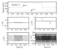
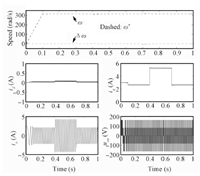
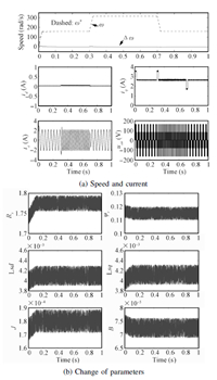
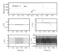
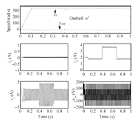
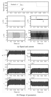
The simulation results are depicted as Figs.1~6. It is obvious from these figures that the current and the speed all are in the given range,which mean the required conditions of the relevant theorems are satisfied. Figs.1~3 shows the simulation results of proposed method 1 under three cases. The simulation results of proposed Method 2 under three cases can be seen in Figs.4~6. In the figures,$\Delta \omega = {\omega ^*} - \omega $ stands the speed error; ${i_a}$ and ${u_{an}}$ are the phase $a$ current and the line to the neutral voltage,respectively.
|
Download:
|
| Fig. 1. The simulation results of proposed Method 1 under Case 1. | |
|
Download:
|
| Fig. 2. The simulation results of proposed Method 1 under Case 2. | |
|
Download:
|
| Fig. 3. The simulation results of proposed Method 1 under Case 3. | |
|
Download:
|
| Fig. 4. The simulation results of proposed Method 2 under Case 1. | |
|
Download:
|
| Fig. 5. The simulation results of proposed Method 2 under Case 2. | |
|
Download:
|
| Fig. 6. The simulation results of proposed Method 2 under Case 3. | |
Figs.1 and 4 show that the speed of PMSM can quickly track the desired speed and its change under the control of proposed Methods 1 and 2,respectively. These reflect the two methods have good tracking performance. it is obvious from Figs.2 and 5 that the proposed control Methods 1 and 2 can make the system effectively resist the load disturbance. Figs.3 and 4 reflect that although the parameters of PMSM change with time,the two proposed control methods can make the speed of motor track the desired speed,which comprehensively verify the control performance of the two methods. Comparing Figs.1~3 and Figs.4~6,we can conclude that the two control methods have similar control performance. Moreover,from these cases,we know that the load information is not needed in the two proposed controllers,which means the two proposed control strategies can deal with the load uncertainty.
Ⅴ. CONCLUSIONSIn this paper,a novel state equation of PMSMs has been obtained via the suitable choice of state variables. Based on the state equation,robust controllers of PMSMs have been developed via interval matrix and PI control idea. In terms of bilinear matrix inequations,sufficient conditions for the existence of the robust controllers have been derived. The proposed controllers can deal with load uncertainty and resist disturbances. In order to demonstrate the effectiveness of proposed control methods,computer simulations have been carried out via Matlab/Simulink. Simulation results have explained the proposed control methods have good control performance.
| [1] | Yang S S, Zhong Y S. Robust speed tracking of permanent magnet synchronous motor servo systems by equivalent disturbance attenuation. IET Control Theory Applications, 2007, 1(3):595-603 |
| [2] | Corradini M L, Ippoliti G, Longhi S, Orlando G. A quasisliding mode approach for robust control and speed estimation of PM synchronous motors. IEEE Transactions on Industrial Electronics, 2012, 59(2):1096-1104 |
| [3] | Choi H H, Vu N T T, Jung J W. Digital implementation of an adaptive speed regulator for a PMSM. IEEE Transactions on Power Electronics, 2011, 26(1):3-8 |
| [4] | Underwood S J, Husain I. Online parameter estimation and adaptive control of permanent-magnet synchronous machines. IEEE Transactions on Industrial Electronics, 2010, 57(7):2345-2443 |
| [5] | Zhu H, Xiao X, Li Y D. Torque ripple reduction of the torque predictive control scheme for permanent-magnet synchronous motors. IEEE Transactions on Industrial Electronics, 2012, 59(2):871-877 |
| [6] | Liu H X, Li S H. Speed control for PMSM servo system using predictive functional control and extended state observer. IEEE Transactions on Industrial Electronics, 2012, 59(2):1171-1183 |
| [7] | Jin H Z, Lee J M. An RMRAC current regulator for permanentmagnet synchronous motor based on statistical model interpretation. IEEE Transactions on Industrial Electronics, 2009, 56(1):169-177 |
| [8] | Hamida M A, Leon J D, Glumineau A, Boisliveau R. An adaptive interconnected observer for sensorless control of PM synchronous motors with online parameter identification. IEEE Transactions on Industrial Electronics, 2013, 60(2):739-747 |
| [9] | Yue X, Vilathgamuwa D M, Tseng K J. Observer-based robust adaptive control of PMSM with initial rotor position uncertainty. IEEE Transactions on Industry Applications, 2003, 39(3):645-656 |
| [10] | Choi H H, Jung J W. Discrete-time fuzzy speed regulator design for PM synchronous motor. IEEE Transactions on Industrial Electronics, 2013, 60(2):600-607 |
| [11] | Chaou H, Sicard P. Adaptive fuzzy logic control of permanent magnet synchronous machines with nonlinear friction. IEEE Transactions on Industrial Electronics, 2012, 59(2):1123-1133 |
| [12] | Leu V Q, Choi H H, Jung J W. Fuzzy sliding mode speed controller for PM synchronous motors with a load torque observer. IEEE Transactions on Power Electronics, 2012, 27(3):1530-1539 |
| [13] | Liu G H, Cheng L L, Zhao W X, Jiang Y, Qu L. Internal model control of permanent magnet synchronous motor using support vector machine generalized inverse. IEEE Transactions on Industrial Informatics, 2013, 9(2):890-898 |
| [14] | Cheng B, Tesch T R. Torque feedforward control technique for permanent-magnet synchronous motors. IEEE Transactions on Industrial Electronics, 2010, 57(3):969-974 |
| [15] | Do T D, Choi H H, Jung J W. SDRE-based near optimal control system design for PM synchronous motor. IEEE Transactions on Industrial Electronics, 2012, 59(11):4063-4074 |
| [16] | Wai R J. Hybrid fuzzy neural-network control for nonlinear motor-toggle servomechanism. IEEE Transactions on Control Systems Technology, 2002, 10(4):519-532 |
| [17] | Lu J G, Chen Y Q. Robust stability and stabilization of fractional-order interval systems with the fractional order α:the 0≤α≤1 case. IEEE Transactions on Automatic Control, 2010, 55(1):152-158 |
| [18] | Guo L. H∞ output feedback control for delay systems with nonlinear and parametric uncertainties. IEE Proceedings-Control Theory and Applications, 2002, 149(3):226-236 |
| [19] | Zhao L, Ham C, Han Q, Wu T X, Zheng L, Sundaram K, Kapat J, Chow L. Design of optimal digital controller for stable super-high-speed permanent-magnet synchronous motor. IEE Proceedings-Electric Power Applications, 2006, 153(2):213-218 |
| [20] | Chen B S, Yuan Y, Chen W, Ni G, Chen M. Electric Drive Automatic Control System:Motion Control System (Third Edition). Beijing, China:China Machine Press, 2003(in Chinese) |
| [21] | Khargonekar P, Petersen I, Zhou K M. Robust stabilization of uncertain linear systems:quadratic stabilizability and H∞ control theory. IEEE Transactions on Automatic Control, 1990, 35(3):256-361 |
| [22] | Boyd S, Ghaoui L, Balakrishnan V. Linear Matrix Inequalities in System and Control Theory. Philadelphia, PA:SIAM, 1994. |
| [23] | Mao W J, Chu J. Quadratic stability and stabilization of dynamic interval systems. IEEE Transactions on Automatic Control, 2003, 48(6):1007-1012 |
 2015, Vol.2


