2. NASA Ames Research Center, Moffet Field, CA 94035, USA
MANY real-world engineering problems are distributed in nature and can be described by a set of partial differential equations (PDEs). A lumped parameter approximation is often adequate in many cases such as in the study of stability and control of an airplane,rockets,and missiles,and design of cooling systems etc. There is a broad class of problems,however, (e.g.,fluid flow,aeroelastic structure,etc.) for which one must take the spatial distribution into account. These systems are also characterized as distributed parameter systems (DPS). Analysis and controller design for such systems are often far more complex than for the lumped parameter systems (which are governed by a finite number of ordinary differential equations).
Control of distributed parameter systems has been studied in the past both from mathematical as well as engineering points of view. An interesting but brief historical perspective of the control of such systems can be found in [1]. In a broad sense,control design techniques for distributed parameter system can be classified as either "approximate-then-design (ATD)" or "deign-then-approximate (DTA)" approaches. An interested reader can refer to [2] for discussion on the relative merits and limitations of the two approaches. In the DTA approach,the usual procedure is to use infinite-dimensional operator theory to design the control in the infinite-dimensional space[3]. While there are many advantages; these approaches are mainly confined to the linear systems and have difficulties in control implementation through an infinite dimensional operator. To overcome this difficulty in an interesting way,the study in [4] presents two techniques of control design based on the DTA approach. One combines the method of dynamic inversion with variational optimization theory which is applicable when there is a continuous actuator in the spatial domain. The other technique,which can be applied when there are a number of discrete actuators located at distinct places in the spatial domain,combines dynamic inversion with static optimization theory.
In the ATD approach,the idea is to first design a low-dimensional reduced model which retains the dominant modes of the system. A popular DPS analysis and synthesis technique is to use orthogonal basis functions in a Galerkin procedure to first create an approximate finite-dimensional system of ordinary differential equations (ODEs). This lumped parameter model is then used for controller design. If arbitrary basis functions (e.g.,Fourier and Chebyshev polynomial) are used in the Galerkin procedure,they can result in a high-dimensional ODE system. A better and powerful basis function design is obtained when the proper orthogonal decomposition (POD) technique is used with a Galerkin approximation. In the POD technique,a set of problem oriented basis functions is first obtained by generating a set of snap-shot solutions through simulations or from the actual process. Using these orthogonal basis functions in a Galerkin procedure,a low-dimensional ODE system can be developed. The same idea is used in this study to obtain a lumped parameter model. Interested readers can further refer to [5, 6, 7, 8].
After obtaining a lumped parameter model,the issue of optimal control synthesis should be addressed next. It is well known that the dynamic programming formulation offers the most comprehensive solution approach to nonlinear optimal control in a state feedback form[9, 10]. However,solving the associated Hamilton-Jacobi-Bellman (HJB) equation demands a large number of computations and storage space dedicated to this purpose. Werbos[11] proposed a means to get around this numerical complexity by using "approximate dynamic programming" (ADP) formulations. This ADP process,through the nonlinear function approximation capabilities of neural networks,overcomes the computational complexity that plagued the dynamic programming formulation of optimal control problems. More importantly,this solution can be implemented online,since the control computation requires a few multiplications of the network weights which are trained offline. This technique was used in [12] to solve an aircraft control problem. The solution to the ADP formulation is obtained through a dual neural network approach called "Adaptive critics (AC)". In one version of the AC approach,called the heuristic dynamic programming (HDP),one network,namely the action network represents the mapping between the state and control variables while a second network,called the critic network, represents the mapping between the state and the cost function to be minimized. In the dual heuristic programming (DHP) class with ACs, while the action network remains the same as the HDP,the critic network outputs the co-states with the current states as inputs. A single-network-adaptive-critic (SNAC)[13] was developed to eliminate the need for the second network. Advantages of SNAC include considerable decrease in the offline training effort and simplicity of the online implementation that results in less computational resources and storage. In [14],SNAC was implemented on a distributed parameter model for beaver population control. Another application was presented in [15],in which a robust optimal controller was designed to obtain a desired temperature profile of a re-entry vehicle. A heat application problem was solved in [16].
In this paper,the POD technique and approximate dynamic programming are combined to develop a generic control design approach for a class of nonlinear DPS. System with continuous control actuation will be studied in terms of performance analysis. This approach is applied to control the heave dynamics of an aircraft$'$s flexible wing model. This application comes under the field of aeroelastic studies,which deals with the interaction of structural,inertial and aerodynamic forces. Current model is inspired from a "beam-mass-beam (BMB)" system[17- 18],where two Euler-Bernoulli beams connected to rigid mass represent a flexible wing with fuselage. A schematic of BMB system is shown in Fig. 1.

|
Download:
|
| Fig. 1. Aircraft flexible wing model (BMB system). | |
In real world applications,the physical parameters used in the PDE models are often unknown. Online adaptive controllers can be used to estimate these parametric uncertainties and mitigate the loss in performance. Although the theory of adaptive controllers for finite dimensional systems is well developed[19, 20],for PDE$'$s adaptive controllers exist only for a few classes of problems. Most of the available adaptive controls schemes are for parabolic type PDE$'$s. See [21, 22, 23] for some of the adaptive control techniques proposed for linear parabolic systems. In general,the techniques for adaptive control of PDE$'$s can be classified as reference model based or identifier based. The objective of model reference adaptive control techniques is to determine a feedback control law,which directs the state to follow a reference model asymptotically. On the other hand, identifier based techniques estimate the unknown system parameters using an approximate model of the system[24, 25],and use them in the design of adaptive controllers. In this paper,an identifier based adaptive control technique is proposed which can handle matched parametric uncertainties. The structure of the PDEs governing the dynamics of the flexible aircraft wings lends itself to use a parabolic type passive identifier for estimating the uncertainties. The proposed identifier assumes that all system states are measured. Simulations are carried out by assuming parametric uncertainties which can make the inherently stable BMB system unstable.
Rest of the paper is organized as follows: Section II describes the class of DPS problems and its control objective. Section III discusses the process of obtaining a finite-dimensional approximate model using the POD technique. Section IV briefly describes the optimal control synthesis using SNAC. Section V discusses the problem of aircraft flexible wing model. In Section VI,the theory behind augmenting the SNAC controller with an adaptive controller is discussed. Simulation results are presented in Section VII. Conclusions are drawn in Section VIII.
Ⅱ. PROBLEM DESCRIPTIONThe class of PDEs considered in this paper describing second-order system dynamics with appropriate boundary conditions is given by
| \begin{align} & \dot {x}_1 =f_1 \left( {x,x^1,x^2,\cdots} \right),\notag \\ & \dot {x}_2 =f_2 \left( {x,x^1,x^2,\cdots} \right)+g\left( {x,x^1,x^2,\cdots} \right)u, \end{align} | (1) |
The objective is to find the optimal control $u(t,y)$ which minimizes the quadratic cost function,defined as
| \begin{align} \label{eq2} J=\frac{1}{2}\int\nolimits_{t_o}^{t_f \to \infty } {\int\nolimits_{y_o}^{y_f} {\left( {x^{\rm T}qx+ru^2} \right){\rm d}y} {\rm d}t}, \end{align} | (2) |
This section discusses the development of a low order finite dimensional model for control synthesis.
A. Generating Snapshot SolutionsSnapshot solution generation is one of the important steps in generating problem oriented basis functions. A low-order lumped parameter approximate model is obtained using these basis functions by applying the Galerkin procedure. The first step is to generate the snapshot solutions. These are representative solutions of the states at arbitrary instants of time that one may possibly encounter when the system operates. Intuition must be used to determine at what time the snapshots must be taken in order to obtain linearly independent basis function[16].
B. Proper Orthogonal Decomposition (POD): a Brief ReviewPOD is a technique for determining an optimal set of basis functions which results in a low order finite dimensional model for an infinite dimensional system when used in a Galerkin procedure. The set of snapshot solutions obtained by the method described in Section III-A is used to generate the basis functions.
Let $\{x_i \left( y \right):1\le i\le N,y\in \left[{0,l} \right]\}$ be a set of $N$ snapshot solutions of a system over the domain $\left[{0,l} \right]$ at arbitrary instants of time. The goal of the POD technique is to design a coherent structure that has the largest mean square projection on the snapshots,i.e.,to find a set of basis function $\varphi $ such that $I$ is maximized.
| \begin{align} \label{eq3} I=\frac{1}{N}\mathop \sum \limits_{i=1}^N \frac{\left\langle {x_i ,\varphi } \right\rangle ^2}{\left\langle {\varphi ,\varphi } \right\rangle} \end{align} | (3) |
| \begin{equation} \label{eq4} \varphi =\sum\limits_{i=1}^N {p_i x_i }, \end{equation} | (4) |
1) Construct an eigenvalue problem
| \begin{equation} \label{eq5} CP=\lambda P, \end{equation} | (5) |
2) Obtain $N$ eigenvalues and corresponding eigenvectors of $C$. Note that $C$ is symmetric and hence the eigenvalues are real. Moreover,it can be shown [27] that it is a positive semi-definite matrix as well. So,all of the eigenvalues are non-negative.
3) Arrange eigenvalues $\left[ \bar{\lambda}_1,\bar{\lambda}_2,\cdots,\bar{\lambda}_N\right]$ of matrix $C$ in descending order such that $ \bar{\lambda}_1\geq\bar{\lambda}_2\geq\cdots\geq\bar{\lambda}_N\geq0$.
4) Find the corresponding eigenvectors,let \begin{align*} P^1=&\left[{p_1^1 ,p_2^1,\cdots,p_N^1 } \right]^{\rm T},\\ P^2=&\left[{p_1^2 ,p_2^2,\cdots,p_N^2 } \right]^{\rm T}, \\ \qquad \qquad \qquad \vdots \\ P^N=&\left[{p_1^N ,p_2^N,\cdots,p_N^N } \right]^{\rm T}. \end{align*}
5) Normalize the eigenvectors to satisfy \[ \left\langle {P^l,P^l} \right\rangle =\left( {P^l} \right)^{\rm T}P^l=\frac{1}{N\lambda _l }. \] This will ensure that the POD basis functions are orthonormal.
6) Truncate the eigen-spectrum such that $$\mathop \sum \limits_{j=1}^{\tilde{N}} {\bar\lambda }_j\cong\sum \limits_{j=1}^{{ N}} {\bar\lambda }_j.$$
Usually,it turns out that ${\tilde{N}}\ll N$.
7) Finally,construct the ${\tilde{N}}$ basis functions as
| \begin{equation} \label{eq6} \varphi _j \left( y \right)=\mathop \sum \limits_{i=1}^N p_i^j x_i \left( y \right),j=1,2,\cdots ,\tilde{N}. \end{equation} | (6) |
The method of snapshot generation and development for proper orthogonal decomposition based model reduction,as applicable to the present problem,are covered in detail in [28, 29]. For detailed discussion of this procedure,an interested reader can refer to [8, 27, 30]. An important property of the POD technique is that basis functions capture the greatest possible energy on an average and therefore,the POD technique leads to an optimally reduced system in general. For a proof of this claim along with some other important properties,the reader can refer to [8].
C. Lumped Parameter SystemThe reduction of the infinite-dimensional problem to a finite set of ordinary differential equations and the related cost function are explained in this subsection. After obtaining the basis functions,state $x\left( {t,y} \right)$ and control $u\left( {t,y} \right)$ are expanded as follows: \[ x\left( {t,y} \right)\approx \mathop \sum \limits_{j=1}^{\tilde{N}} \hat{x}_j(t)\varphi_j(y), \] \[ u\left( {t,y} \right)\approx \mathop \sum \limits_{j=1}^{\tilde{N}} \hat{u}_j(t)\varphi_j(y), \] here $\hat{x}_j(t)$ and $\hat{u}_j(t)~(j=1,2,\cdots,{\tilde{N}})$ are the auxiliary state and control variables of the lumped parameter model. One can notice that both $x\left( {t,y} \right)$ and $u\left( {t,y} \right)$ have the same basis functions. We assume that state feedback controller spans a subspace of the state variables and hence,the basis functions for the state are assumed to be capable of spanning the controller as well.
For our control problem,the basis functions for states $x_1 $ and $x_2 $ are designed separately. The state variables $x_1 \left( {t,y} \right)$,and $x_2 \left( {t,y} \right)$ can be written in terms of basis functions $\varphi _{1_j } \left( y \right)$ and $\varphi _{2_j } \left( y \right)$,$j=1,2,\cdots,{\tilde{N}}$ respectively as
| \begin{equation} \label{eq7} x_1 \left( {t,y} \right)=\mathop \sum \limits_{j=1}^{\tilde{N}} \hat{x}_{1j}(t)\varphi_{1j}(y),x_2(t,y)=\sum \limits_{j=1}^{\tilde{N}} \hat{x}_{2j}(t)\varphi_{2j}(y). \end{equation} | (7) |
| \begin{equation} \label{eq8} u\left( {t,y} \right)=\mathop \sum \limits_{j=1}^{\tilde{N}} \hat{u}_{1j}(t)\varphi_{1j}(y),+\sum \limits_{j=1}^{\tilde{N}} \hat{u}_{2j}(t)\varphi_{2j}(y). \end{equation} | (8) |
For convenience,we define $\hat{X}_1=[\bar x_{1_1},\cdots,\bar x_{1_{\tilde{N}}}]^{\rm T},\hat{X}_2=[\bar x_{2_1},\cdots,\bar x_{2_{\tilde{N}}}]^{\rm T},\hat{U}_1=[\bar u_{1_1},\cdots,\bar u_{1_{\tilde{N}}}]^{\rm T},\hat{U}_2=[\bar u_{2_1},\cdots,$ $\bar u_{2_{\tilde{N}}}]^{\rm T} $. Next,we discuss finite dimensional approximation of system using Galerkin procedure,please see what is more appropriate. Substituting expansions of state (7) and control (8) in (1),
| \begin{align} &\mathop\sum \limits_{i=1}^{\tilde{N}}\dot{{\hat{x}}}_{1_i} (t)\varphi_{1_i}(y)=\notag\\ &\quad f_1\left(\left[\sum \limits_{i=1}^{\tilde{N}}\hat{x}_{1_i}(t)\varphi_{1_i}(y),\sum \limits_{i=1}^{\tilde{N}}\hat{x}_{2_i}(t)\varphi_{2_i}(y)\right]^{\rm T},\notag\right.\\ &\quad\left.\left[\sum \limits_{i=1}^{\tilde{N}}\hat{x}_{1_i}(t)\varphi_{1_i}^1(y),\sum \limits_{i=1}^{\tilde{N}}\hat{x}_{2_i}(t)\varphi_{2_i}^1(y)\right]^{\rm T},\cdots\right), \end{align} | (9) |
| \begin{align*} &\mathop\sum \limits_{i=1}^{\tilde{N}}\dot{{\hat{x}}}_{2_i} (t)\varphi_{2_i}(y)=\notag\\ & f_2\left(\left[\sum \limits_{i=1}^{\tilde{N}}\hat{x}_{1_i}(t)\varphi_{1_i}(y),\sum \limits_{i=1}^{\tilde{N}}\hat{x}_{2_i}(t)\varphi_{2_i}(y)\right]^{\rm T},\cdots\notag\right)+ \end{align*} \begin{align} &g\left(\left[\sum \limits_{i=1}^{\tilde{N}}\hat{x}_{1_i}(t)\varphi_{1_i}(y),\sum \limits_{i=1}^{\tilde{N}}\hat{x}_{2_i}(t)\varphi_{2_i}(y)\right]^{\rm T},\cdots\right)\times\notag\\ &\left(\sum \limits_{j=1}^{\tilde{N}}\hat{u}_{1_j}(t)\varphi_{1_i}(y)+\sum \limits_{j=1}^{\tilde{N}}\hat{u}_{2_j}(t)\varphi_{2_j}(y)\right). \end{align} | (10) |
Next,taking the Galerkin projection of (9) with $\varphi _{1_j } \left( y \right)$ and of (10) with $\varphi _{2_j } \left( y \right)$ and using the fact that these basis functions are orthonormal,it yields
| \begin{align} \dot{\hat{x}}_{1_j}=\dot{f}_{1_j}(\hat{X}_1,\hat{X}_2),~~j=1,2,\cdots,\tilde{N}, \end{align} | (11) |
| \begin{align} \dot{\hat{x}}_{2_j}=\dot{f}_{2_j}(\hat{X}_1,\hat{X}_2)+\hat{g}_j(\hat{X}_1,\hat{X}_2)[\hat{U}_1,\hat{U}_2]^{\rm T},~~j=1,2,\cdots,\tilde{N}, \end{align} | (12) |
| \begin{align} &\hat{f}_{1j}(\hat{X}_1,\hat{X}_2)=\langle f_1(x,x^1,x^2,\cdots),\varphi_{1_j}\rangle=\notag\\ &\quad\int f_1(x,x^1,x^2,\cdots)\varphi_{1_j}{\rm d}y, \end{align} | (13) |
| \begin{align} &\hat{f}_{2j}(\hat{X}_1,\hat{X}_2)=\langle f_2(x,x^1,x^2,\cdots),\varphi_{2_j}\rangle=\notag\\ &\quad\int f_2(x,x^1,x^2,\cdots)\varphi_{2_j}{\rm d}y, \end{align} | (14) |
| \begin{align} &\hat{g}_{j}(\hat{X}_1,\hat{X}_2)[\hat{U}_1,\hat{U}_2]^{\rm T}=\langle q(x,x^1,x^2,\cdots)u,\varphi_{2_j}\rangle=\notag\\ &\quad\int q(x,x^1,x^2,\cdots)u\varphi_{2_j}{\rm d}y. \end{align} | (15) |
Next,in the cost function (2),the terms can be represented as
| \begin{align} &\int^{y_f}_{y_o}(x^{\rm T}qx){\rm d}y=\notag\\ &\quad \int^{y_f}_{y_o}\left(\left[\sum \limits_{i=1}^{\tilde{N}}\hat{x}_{1_i}(t)\varphi_{1_i}(y),\sum \limits_{i=1}^{\tilde{N}}\hat{x}_{2_i}(t)\varphi_{2_i}(y)\right]\times\notag\right.\\ &\quad q\left.\left[\sum \limits_{i=1}^{\tilde{N}}\hat{x}_{1_i}(t)\varphi_{1_i}(y),\sum \limits_{i=1}^{\tilde{N}}\hat{x}_{2_i}(t)\varphi_{2_i}(y)\right]^{\rm T}\right){\rm d}y,\notag\\ &\qquad\int^{y_f}_{y_o}(x^{\rm T}qx){\rm d}y=[\hat{X}_1^{\rm T}, \hat{X}_2^{\rm T}]Q[\hat{X}_1^{\rm T},\hat{X}_2^{\rm T}]^{\rm T}, \end{align} | (16) |
| \begin{align} &\int^{y_f}_{y_o}(ru^2){\rm d}y=\notag\\ &\quad \int^{y_f}_{y_o}\left(r\left[\sum \limits_{i=1}^{\tilde{N}}\hat{u}_{1_i}(t)\varphi_{1_i}(y)+\sum \limits_{i=1}^{\tilde{N}}\hat{u}_{2_i}(t)\varphi_{2_i}(y)\right]^2\notag\right){\rm d}y,\\ &\qquad\int^{y_f}_{y_o}(ru^2){\rm d}y=[\hat{U}_1^{\rm T}, \hat{U}_2^{\rm T}]R[\hat{U}_1^{\rm T},\hat{U}_2^{\rm T}]^{\rm T} \end{align} | (17) |
Let \begin{align*} &q=\left[{{\begin{array}{*{20}c} {q_{11} } \hfill & {q_{12} } \hfill \\ {q_{21} } \hfill & {q_{22} } \hfill \\ \end{array} }} \right]_{2\times 2},\\ &Q=\left[{{\begin{array}{*{20}c} {Q_{11} } \hfill & {Q_{12} } \hfill \\ {Q_{21} } \hfill & {Q_{22} } \hfill \\ \end{array} }} \right]_{2\tilde{N}\times2\tilde{N}},\\ &R=r\left[{{\begin{array}{*{20}c} {R_{11} } \hfill & {R_{12} } \hfill \\ {R_{21} } \hfill & {R_{22} } \hfill \\ \end{array} }} \right]_{2\tilde{N}\times2\tilde{N}}. \end{align*} where \begin{align*} & R_{11} \left( {i,j} \right)=\int \varphi _{1_i } \left( y \right)\varphi _{1_j } \left( y \right){\rm d}y,\\ & R_{12} \left( {i,j} \right)=\int \varphi _{1_i } \left( y \right)\varphi _{2_j } \left( y \right){\rm d}y,\\ & R_{21} \left( {i,j} \right)=\int \varphi _{2_i } \left( y \right)\varphi _{1_j } \left( y \right){\rm d}y,\\ & R_{22} \left( {i,j} \right)=\int \varphi _{2_i } \left( y \right)\varphi _{2_j } \left( y \right){\rm d}y,\\ & Q_{11} \left( {i,j} \right)=q_{11} R_{11} \left( {i,j} \right),\\ & Q_{12} \left( {i,j} \right)=q_{12} R_{12} \left( {i,j} \right),\\ & Q_{21} \left( {i,j} \right)=q_{21} R_{21} \left( {i,j} \right),\\ & Q_{22} \left( {i,j} \right)=q_{22} R_{22} \left( {i,j} \right),\\ \end{align*} where $i=1,2,\cdots,\tilde{N}$ and $j=1,2,\cdots,\tilde{N}$. Thus the cost function in (2) can be written as
| \begin{align} &J=\frac{1}{2} \int_{t_o }^{t_f \to \infty } \left( \left[ \hat{X}_1^{\rm T},\hat{X}_2^{\rm T} \right]Q \left[\hat{X}_1^{\rm T},\hat{X}_2^{\rm T} \right]^{\rm T}+\right.\notag\\ &\quad \left.\left[\hat{U}_1^{\rm T},\hat{U}_2^{\rm T} \right]R\left[\hat{U}_1^{\rm T},\hat{U}_2^{\rm T} \right]^{\rm T}\right){\rm d}t. \end{align} | (18) |
In this section,a fairly general discussion on optimal control of distributed parameter systems is presented in an ADP framework. Detailed derivations of these conditions can also be found in [11, 12],which are repeated here for the sake of completeness. Since the optimal controller is to be implemented online,the problem is formulated in discrete domain.
A. Problem Description and Optimality ConditionsConsider a system given by
| \begin{align} \hat{X}_{k+1}=F_k(\hat{X}_k,\hat{U}_k), \end{align} | (19) |
| \begin{align} J=\sum \limits_{k=1}^{N-1} \Psi _k (\hat{X}_k,\hat{U}_k), \end{align} | (20) |
| \begin{align} J_k=\sum \limits_{\bar{k}=k}^{N-1} \Psi _{\bar k} (\hat{X}_{\bar k},\hat{U}_{\bar k}). \end{align} | (21) |
| \begin{align} J_k =\Psi _k +J_{k+1}, \end{align} | (22) |
| \begin{align} \lambda _k := \frac{\partial J_k }{\partial \hat{X}_k}. \end{align} | (23) |
Then,the necessary condition for optimality for optimal control is
| \begin{align} \frac{\partial J_k }{\partial \hat{U}_k}=0. \end{align} | (24) |
After some manipulations,the optimal control equation is obtained as
| \begin{align} \left( {\frac{\partial \Psi _k }{\partial \hat{U}_k}} \right)+ \left( {\frac{\partial \hat{X} _{k+1} }{\partial \hat{U}_k}} \right)^{\rm T}\lambda_{k+1}=0. \end{align} | (25) |
By using (23) in the equation above
| \begin{align} \lambda _k =\left( {\frac{\partial \Psi _k }{\partial \hat{X}_k}} \right)+ \left( {\frac{\partial \hat{X} _{k+1} }{\partial \hat{X}_k}} \right)^{\rm T}\lambda_{k+1}. \end{align} | (26) |
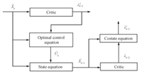
The adaptive-critic synthesis for optimal controller design of a lumped parameter system is discussed in detail in [12]. The core of the technique lies in the iterative training between the critic and action networks. The action network is to capture the relationship between the states and control at stage $k$ and the critic network to capture the relationship between the states and the costates at stage $k$. By contrast,the SNAC captures the relationship between the state at $k$ and the costate at $k+1$ and uses only one neural network. We use this approach to design optimal control for lumped parameter system.
In the present paper,the networks are split internally into $2\hat{N}$ sub-networks,assuming one network for each channel of the costate vector. The input to each sub-network,however,is the entire state vector. This is done to speed up the training process since cross coupling of weights for different components of the output vector are absent in such a framework. The first step of training procedure is state generation for neural network training. Note that the lumped parameter states can be computed from $x\left( {t,y} \right)$ as \begin{align*} \hat{x}_{1_j}(t)=\langle x_1(t,y),\phi_{1_j}(y)\rangle, \end{align*} and \begin{align*} \hat{x}_{2_j}(t)=\langle x_2(t,y),\phi_{2_j}(y)\rangle, \end{align*} where $j=1,2,\cdots ,\tilde{N}$. One can generate a state profile $x\left( {t,y} \right)$ as described in Subsection III-A and then use it to construct the lumped parameter states,which can subsequently be used for training the networks. However,due to the requirement of large number of state profiles,this process would slow down the program significantly. Therefore,an alternative method of generating the lumped parameter state vector for training the network is followed. All generated snapshots are used to get the minimum and values for the individual elements of state vector. Training is first carried out by generating the state close to zero and then the training set is expanded including more data points. Let $[{\hat{X}_{1\min}},\hat{X}_{2\min}]$ and $[ \hat{X}_{1\max},\hat{X}_{2\max}]$ denote the vectors of minimum and maximum values of the elements of $[\hat{X}_{1},\hat{X}_{2}]$. The initial training set is obtained by setting a constant $C_i \in \left[{0,1} \right]$,$C_1 =0.05$ and generating training points in the domain $S_i := C_i [[\hat{X}_{1\min},\hat{X}_{2\min}],[ \hat{X}_{1\max},\hat{X}_{2\max}]]$. Once the network is trained in this set,$C_i $ is changed as $C_i =C_1 +0.05\left( {i-1} \right)$ for $i=2,3,\cdots,$ and the network is trained again. This process is repeated until $C_i =1$.
The steps for training (offline) the critic network which captures the relationships between state at time $k$ and co-state at time $k+1$ are as follows:
1) Fix $C_i $ and generate training domain $S_i$;
2) For each element $\hat{X}_k$ of $S_i $ follow the steps below:
a) Input $\hat{X}_k$ to networks to get $\lambda _{k+1}$. Let us denote it as $\lambda _{k+1}^a$.
b) Calculate $\hat{U}_k$,knowing $\hat{X}_k$ and $\lambda _{k+1} $, from optimal control (25);
c) Get $\hat{X}_{k+1}$ from the state equation (19),using $\hat{X}_k$ and $\hat{U}_k$.
d) Input $\hat{X}_{k+1}$ to the networks to get $\lambda _{k+2} $.
e) Calculate $\lambda _{k+1} $ ,from the costate equation. Denote this as $\lambda _{k+1}^t $.
3) Train the networks,with all $\hat{X}_k$ as inputs and corresponding $\lambda _{k+1}^t $ as outputs.
4) If proper convergence is achieved,stop and revert to step 1, with $S_{i+1} $. If not,go to Step 1) and retrain the network with a new $S_i $.
For faster convergence,one can take a convex combination $\left[ {\beta \lambda _{k+1}^t +\left( {1-\beta } \right)\lambda _{k+1}^a } \right]$ as the target output for training,where $0 < \beta \le 1$ is the learning rate for the neural network training. We set a tolerance value to check the convergence of network. If $\frac{\|\lambda _{k+1}^t -\lambda _{k+1}^a \|_2}{\|\lambda _{k+1}^t \|_2} < $ tolerance then it can be said that the networks have converged. For the present problem,the value of learning rate and tolerance is selected as $0.8$ and $10^{-7}$, respectively.
|
Download:
|
| Fig. 2. Schematic of neural network synthesis. | |
After the offline controller synthesis,the following steps are used for online control computation. Fig. 3 shows the control solution implementation scheme. The offline and online operations are as follows:

|
Download:
|
| Fig. 3. Implementation of control solution. | |
1) Offline operations
a) Train adaptive critic network controller for the system.
2) Online operations
a) Measure the state variables at time $t_k $ across the spatial dimension.
b) Compute the $\hat{X}_k$ using the basis functions
c) Using $\hat{X}_k$ in the neural network,compute the control $\hat{u}_k$.
d) Get the desired control profile $u\left( {t_k ,y} \right)$ from $\hat{U}_k$,using the basis functions.
Ⅴ. A FLEXIBLE WING AIRCRAFT MODELA flexible wing aircraft model is represented by using two Euler-Bernoulli beams connected to a rigid mass as shown in Fig. 1. The BMB system primarily represents the heave dynamics of an aircraft model,which is initially assumed to be in a level flight with its wings straight and the lift force balancing the weight. Any perturbation in the wing$'$s shape (defined by transverse displacement $w\left( {t,y} \right))$ causes a change in the local angle-of-attack distribution over the wing and this in turn leads to perturbation in lift distribution. The objective is to achieve the level flight conditions $\left( {w\left( {t,y} \right)=0} \right)$ using the proposed control action.
The basic dynamic model of BMB is taken from [17] in which a set of only two control actions are considered. In this study, however,the model is further generalized with a continuous form of control action over the left and right beams. First the dynamic model is presented and then the control design is developed. Discussion in Section III is used to obtain a finite dimension approximation and the SNAC described in Section IV is used to design the optimal control action. Transverse displacements for left and right beam are described by $w_L \left( {t,y} \right)$ and $w_R \left( {t,y} \right)$,respectively.
Dynamic equation for the left beam is given as
| \begin{align} & \rho a\frac{\partial ^2w_L \left( {t,y} \right)}{\partial t^2}+EI\frac{\partial ^4w_L \left( {t,y} \right)}{\partial y^4}+\notag\\ &\quad\gamma _1 \frac{\partial w_L \left( {t,y} \right)}{\partial t}+\gamma _2 I\frac{\partial ^5w_L \left( {t,y} \right)}{\partial t\partial y^4}=\notag\\ &\quad-\frac{\Delta L\left( {t,y} \right)}{\frac{l}{2}}+b_L \left( y \right)u_L \left( {t,y} \right), \end{align} | (27) |
| \begin{align} &\rho a\frac{\partial ^2w_R \left( {t,y} \right)}{\partial t^2}+EI\frac{\partial ^4w_R \left( {t,y} \right)}{\partial y^4}+\notag\\ &\quad\gamma _1 \frac{\partial w_R \left( {t,y} \right)}{\partial t}+\gamma _2 I\frac{\partial ^5w_R \left( {t,y} \right)}{\partial t\partial y^4}=\notag\\ &\quad-\frac{\Delta L\left( {t,y} \right)}{\frac{l}{2}}+b_R \left( y \right)u_R \left( {t,y} \right), \end{align} | (28) |
| \begin{align} &EI\frac{\partial ^3w_R \left( {t,l} \right)}{\partial y^3}+\gamma _2 I\frac{\partial ^4w_R \left( {t,l} \right)}{\partial t\partial y^3}=0,\notag\\ & w_L \left( {t,\frac{l}{2}} \right)=w_R \left( {t,\frac{l}{2}} \right),\notag\\ &\frac{\partial w_L \left( {t,\frac{l}{2}} \right)}{\partial y}=\frac{\partial w_R \left( {t,\frac{l}{2}} \right)}{\partial y}. \end{align} | (29) |
| \begin{align} & EI\frac{\partial ^3w_L \left( {t,\frac{l}{2}} \right)}{\partial y^3}+\gamma _2 I\frac{\partial ^4w_L \left( {t,\frac{l}{2}} \right)}{\partial t\partial y^3}-\notag\\ &\quad EI\frac{\partial ^3w_R \left( {t,\frac{l}{2}} \right)}{\partial y^3}-\gamma _2 I\frac{\partial ^4w_R \left( {t,\frac{l}{2}} \right)}{\partial t\partial y^3}=m\frac{\partial ^2w_L \left( {t,\frac{l}{2}} \right)}{\partial t^2},\notag\\ & EI\frac{\partial ^2w_L \left( {t,\frac{l}{2}} \right)}{\partial y^2}+\gamma _2 I\frac{\partial ^3w_L \left( {t,\frac{l}{2}} \right)}{\partial t\partial y^2}-\notag\\ &\quad EI\frac{\partial ^2w_R \left( {t,\frac{l}{2}} \right)}{\partial y^2}-\gamma _2 I\frac{\partial ^3w_R \left( {t,\frac{l}{2}} \right)}{\partial t\partial y^2}=I_Z \frac{\partial ^3w_R \left( {t,\frac{l}{2}} \right)}{\partial t^2\partial y}, \end{align} | (30) |
| \begin{align} & w_L \left( {0,y} \right)=f_L \left( y \right),\notag\\ &\frac{\partial w_L }{\partial t}\left( {0,y} \right)=g_L \left( y \right), \end{align} | (31) |
| \begin{align}& w_R \left( {0,y} \right)=f_R \left( y \right),\notag\\ &\frac{\partial w_R }{\partial t}\left( {0,y} \right)=g_R \left( y \right), \end{align} | (32) |
| \begin{align} & w_1 \left( {t,y} \right)= w_L \left( {t,y} \right),\notag\\ & w_2 \left( {t,y} \right)= \frac{\partial w_L \left( {t,y} \right)}{\partial t}, \end{align} | (33) |
| \begin{align} &\frac{\partial w_1 \left( {t,y} \right)}{\partial t}=w_2 \left( {t,y}\right),\notag\\ & \frac{\partial w_2 \left( {t,y} \right)}{\partial t}=-\frac{EI}{\rho a}\frac{\partial ^4w_1 \left( {t,y} \right)}{\partial y^4}-\frac{\gamma _1 }{\rho a}w_2 \left( {t,y} \right)-\notag\\ &\quad\frac{\gamma _2 I}{\rho a}\frac{\partial ^4w_2 \left( {t,y} \right)}{\partial y^4}-\frac{\Delta L\left( {t,y} \right)}{\frac{l\rho a}{2}}+\frac{b\left( y \right)u\left( {t,y} \right)}{\rho a}. \end{align} | (34) |
Boundary conditions (29) remain the same and conditions at middle point are derived:
| \begin{align} & EI\frac{\partial ^3w_1 \left( {t,\frac{l}{2}} \right)}{\partial y^3}+\gamma _2 I\frac{\partial ^3w_2 \left( {t,\frac{l}{2}} \right)}{\partial y^3}=\notag\\ &\quad\frac{m}{2}\frac{\partial w_2 \left( {t,\frac{l}{2}} \right)}{\partial t},\notag\\ & EI\frac{\partial ^2w_1 \left( {t,\frac{l}{2}} \right)}{\partial y^3}+\gamma _2 I\frac{\partial ^2w_2 \left( {t,\frac{l}{2}} \right)}{\partial y^3}=0. \end{align} | (35) |
The state variables $w_1 \left( {t,y} \right)$,$w_2 \left( {t,y} \right)$ and control variable $u\left( {t,y} \right)$ can be written in terms of basis functions as
| \begin{align} &w_1 \left( {t,y} \right)= \sum \limits_{j=1}^{\tilde{N}} \hat{w}_{1_j}(t)\phi_{1_j}(y),\notag\\ &w_2 \left( {t,y} \right)= \sum \limits_{j=1}^{\tilde{N}} \hat{w}_{2_j}(t)\phi_{2_j}(y), \end{align} | (36) |
| \begin{align} & u\left( {t,y} \right)= \sum \limits_{j=1}^{\tilde{N}} \hat{u}_{1_j}(t)\phi_{1_j}(y)+\sum \limits_{j=1}^{\tilde{N}} \hat{u}_{2_j}(t)\phi_{2_j}(y) \end{align} | (37) |
| \begin{align} & \dot{\hat{w}}_{1_j} =\mathop \sum \limits_{i=1}^{\tilde{N}} \left( \int_{y=0}^{\frac{l}{2}} \varphi _{2_i} \varphi _{1_j} {\rm d}y \right)\hat{w}_{2_i},\notag\\ &\dot{\hat{w}}_{2_j} =-\frac{EI}{\rho a}\mathop \sum \limits_{i=1}^{\tilde{N}} \left( \int_{y=0}^{\frac{l}{2}} \varphi _{1_i}^2 \varphi _{2_j}^2 {\rm d}y \right)\hat{w}_{1_i}-\notag\\ &\quad\frac{\gamma_2I}{\rho a}\mathop \sum \limits_{i=1}^{\tilde{N}} \left( \int_{y=0}^{\frac{l}{2}} \varphi _{2_i}^2 \varphi _{2_j}^2 {\rm d}y \right)\hat{w}_{2_i}-\notag\\ &\quad \frac{\gamma_1}{\rho a}\hat{w}_{2_j} \int_{y=0}^{\frac{l}{2}} \frac{\Delta L(t,y)}{\frac{l\rho a}{2}}\varphi _{2_i} {\rm d}y +\notag\\ &\quad \frac{1}{\rho a}\mathop \sum \limits_{i=1}^{\tilde{N}} \left( \int_{y=0}^{\frac{l}{2}} b(y)\varphi _{1_i} \varphi _{2_j} {\rm d}y \right)\hat{u}_{1_i}+\notag\\ &\quad \frac{1}{\rho a}\mathop \sum \limits_{i=1}^{\tilde{N}} \left( \int_{y=0}^{\frac{l}{2}} b(y)\varphi _{2_i} \varphi _{2_j} {\rm d}y \right)\hat{u}_{2_i}+\notag\\ &\quad\left.\frac{1}{\rho a}[(EIw_2^2+\gamma_2Iw_2^2)\varphi_{2_j}^2]\right|_{\frac{l}{2}}-\notag\\ &\quad\left.\frac{1}{\rho a}[(EIw_1^3+\gamma_2Iw_2^3)\varphi_{2_j}]\right|_{\frac{l}{2}}. \end{align} | (38) |
Notice the superscript as defined in Section II-A. $\Delta L\left( {t,y} \right)$ is the change in the lift distribution from the equilibrium position. The following expression for $\Delta L\left( {t,y} \right)$is assumed:
| \begin{align} \Delta L\left( {t,y} \right)=\frac{1}{2}\rho _a V_o^2 cC_{l_\alpha } \Delta \alpha, \end{align} | (39) |
| \begin{align} \Delta \alpha =\sin ^{-1}\left( {\frac{w_2 }{V_0 }} \right). \end{align} | (40) |
| \begin{align} \Delta \alpha \approx \frac{w_2 }{V}+\frac{1}{6}\left( {\frac{w_2 }{V_0 }} \right)^3 \end{align} | (41) |
| \begin{align*} & \dot{\hat{w}}_{2_j} =-\frac{EI}{\rho a}\mathop \sum \limits_{i=1}^{\tilde{N}} \left( \int _{y=0}^\frac{l}{2} \varphi _{1_i} ^2 \varphi _{2_j} ^2 {\rm d}y \right)\hat{w}_{1_i}-\notag \\ &\quad\frac{\gamma_2I}{\rho a}\mathop \sum \limits_{i=1}^{\tilde{N}} \left( \int _{y=0}^\frac{l}{2} \varphi _{2_i} ^2 \varphi _{2_j} ^2 {\rm d}y \right)\hat{w}_{2_i}-\frac{\gamma_1I}{\rho a}\hat{w}_{2_j} -\\ &\quad \frac{\rho_aV_o^2cC_{l_\alpha}}{l\rho a}\mathop \int _{y=0}^\frac{l}{2} \left(\frac{w_2}{V_0}+\frac{1}{6}\left(\frac{w_2}{V_0}\right)^3\right)\varphi_{2_j}{\rm d}y+\\ &\quad\frac{1}{\rho a}\mathop \sum \limits_{i=1}^{\tilde{N}} \left( \int _{y=0}^\frac{l}{2}b(y) \varphi _{1_i} \varphi _{2_j} {\rm d}y \right)\hat{u}_{1_i}+ \end{align*} \begin{align} &\quad\frac{1}{\rho a}\mathop \sum \limits_{i=1}^{\tilde{N}} \left( \int _{y=0}^\frac{l}{2}b(y) \varphi _{2_i} \varphi _{2_j} {\rm d}y \right)\hat{u}_{2_i}-\notag\\ &\quad\frac{m}{2\rho a}\left.\left[\left(\mathop \sum \limits_{j=1}^{\tilde{N}} \dot{\hat{w}}_{2_i}(t) \varphi _{2_i}(y) \right)\varphi_{2_j}\right]\right|_\frac{l}{2},\notag\\ & \dot{\hat{w}}_{2_j} =-\frac{EI}{\rho a}\mathop \sum \limits_{i=1}^{\tilde{N}} \left( \int _{y=0}^\frac{l}{2} \varphi _{1_i} ^2 \varphi _{2_j} ^2 {\rm d}y \right)\hat{w}_{1_i}-\notag \\ &\quad\frac{\gamma_2I}{\rho a}\mathop \sum \limits_{i=1}^{\tilde{N}} \left( \int _{y=0}^\frac{l}{2} \varphi _{2_i} ^2 \varphi _{2_j} ^2 {\rm d}y \right)\hat{w}_{2_i}-\frac{\gamma_1}{\rho a}\hat{w}_{2_j} -\notag\\ &\quad \frac{\rho_aV_o^2cC_{l_\alpha}}{l\rho a}\hat{w}_{2_j}-\frac{\rho_acC_{l_\alpha}}{6l\rho aV_0}\times\notag\\ &\quad \mathop \int _{y=0}^\frac{l}{2}\times\left[\sum\limits_{k_1+k_2+\cdots+k_{\tilde{N}}=3}\left(\frac{3!}{k_1!k_2!\cdots k_{\tilde{N}}!}\right)\right.\notag\\ &\quad \left.\prod\limits_{i=1}^{\tilde{N}}(\hat{w}_{2_i}(t)\varphi_{2_i}(y))^{k_i}\right]\times\notag\\ &\quad\varphi_{2_j}{\rm d}y+\frac{1}{\rho a}\mathop \sum \limits_{i=1}^{\tilde{N}} \left( \int _{y=0}^\frac{l}{2}b(y) \varphi _{1_i} \varphi _{2_j} {\rm d}y \right)\hat{u}_{1_i}+\notag\\ &\quad\frac{1}{\rho a}\mathop \sum \limits_{i=1}^{\tilde{N}} \left( \int _{y=0}^\frac{l}{2}b(y) \varphi _{2_i} \varphi _{2_j} {\rm d}y \right)\hat{u}_{2_i}-\notag\\ &\quad\frac{m}{2\rho a}\left.\left[\left(\mathop \sum \limits_{j=1}^{\tilde{N}} \dot{\hat{w}}_{2_i}(t) \varphi _{2_i}(y) \right)\varphi_{2_j}\right]\right|_\frac{l}{2}. \end{align} | (42) |
Note that the first equation of (38) and (42) are in the form of (11) and (12),respectively.
Ⅵ. SNAC CONTROLLER AUGMENTED WITH ADAPTIVE CONTROLLERTo compensate for the real life uncertainties arising out of unknown physical parameters in the system,an adaptive controller using a passive identifier is proposed. Let the actual flexible aircraft system model be in the form given in (43). Note that (43) has an extra term $h\left( {w_1 ,w_2 } \right)$ as compared to (34) which represents the uncertainties.
| \begin{align} & \frac{\partial w_2 \left( {t,y} \right)}{\partial t}=-\frac{EI}{\rho a}\frac{\partial ^4w_1 \left( {t,y} \right)}{\partial y^4}-\frac{\gamma _1 }{\rho a}w_2 \left( {t,y} \right)-\notag\\ &\quad\frac{\gamma _2 I}{\rho a}\frac{\partial ^4w_2 \left( {t,y} \right)}{\partial y^4}-\frac{\Delta L\left( {t,y} \right)}{\frac{l\rho a}{2}}+\notag\\ &\quad\frac{b\left( y \right)u\left( {t,y} \right)}{\rho a}+h\left( {w_1 ,w_2 } \right). \end{align} | (43) |
| \begin{align} h\left( {w_1 ,w_2 } \right)=W_N^{\rm T} \sigma \left( {w_1 ,w_2 } \right), \end{align} | (44) |
| \begin{align} & \frac{\partial \bar{w}_2 \left( {t,y} \right)}{\partial t}=-\frac{EI}{\rho a}\frac{\partial ^4w_1 \left( {t,y} \right)}{\partial y^4}-\frac{\gamma _1 }{\rho a}w_2 \left( {t,y} \right)-\notag\\ &\quad\frac{\gamma _2 I}{\rho a}\frac{\partial ^4w_2 \left( {t,y} \right)}{\partial y^4}-\frac{\Delta L\left( {t,y} \right)}{\frac{l\rho a}{2}}+\notag\\ &\quad\frac{b\left( y \right)u\left( {t,y} \right)}{\rho a}+\hat{W}_N^{\rm T}\sigma(w_1,w_2)+a_2\left( {w_2-\hat{w}_2 } \right), \end{align} | (45) |
| \begin{align} \frac{\partial e\left( {t,y} \right)}{\partial t}=-a_2 e\left( {t,y} \right)+\hat{W}_N^{\rm T}\sigma(w_1,w_2), \end{align} | (46) |
| \begin{align} V=\frac{1}{2}\left( \mathop \int _0^l e\left( {t,y} \right)^2{\rm d}y+\tilde{W}_N^{\rm T}F^{-1}\tilde{W}_N \right). \end{align} | (47) |
The time derivative of the Lyapunov equation (47) is written as
| \begin{align} \dot{V}=\mathop\int_0^l e\left( {t,y} \right)\frac{\partial e}{\partial t}{\rm d}y+\tilde{W}_N^{\rm T}F^{-1}{\dot{\tilde{W}}}_N. \end{align} | (48) |
| \begin{align} &\dot{V}=-a_2 \mathop \int _0^l e\left( {t,y} \right)^2{\rm d}y+\int _0^l e\left( {t,y} \right) \tilde{W}_N^{\rm T}\sigma (w_1,w_2){\rm d}y-\notag\\ &\quad\tilde{W}_N^{\rm T}F^{-1}\dot{\tilde{W}}_N. \end{align} | (49) |
| \begin{align} \dot{{{\tilde{W}}}}_N =F\mathop \int _0^l e\left( {t,y} \right)\sigma \left( {w_1 ,w_2 } \right){\rm d}y. \end{align} | (50) |
| \begin{align} \dot{{V}} =-a_2F\mathop \int _0^l e\left( {t,y} \right)^2{\rm d}y\leq 0. \end{align} | (51) |
Numerical simulations are performed in Matlab. All the simulation parameter values used in this study for flexible beam problem are listed in Tables I and II. Ten basis functions (for each state) were found to be sufficient to "approximately" describe the flexible model in finite-dimensions. These basis functions were obtained from 3 840 snap-shots,which are captured by simulating the BMB system with random initial state profiles. Here,the term "approximately" indicates that these basis functions are able to capture nearly 99 % of energy (given by (3)) in the beam displacement and the rate of the beam displacement. Using these basis functions,a lumped parameter model is obtained and the controller is designed using SNAC. The following basis functions were used in the linear-in-parameter neural network for each costate of the lumped parameter model: \begin{align*} &[\hat{w}_{1_1},\hat{w}_{1_2},\cdots,\hat{w}_{1_{10}},\hat{w}_{2_1},\cdots,\\ &\quad\hat{w}_{2_{10}},(\hat{w}_{2_1})^2,(\hat{w}_{2_1})^3,(\hat{w}_{2_1})^4, \hat{w}_{1_1}\hat{w}_{2_1}]_{24\times1}^{\rm T} \end{align*}
|
|
TABLE Ⅰ SYSTEM PARAMETERS FOR FLEXIBLE BEAM PROBLEM |
|
|
TABLE Ⅱ NUMERICAL PARAMETERS FPR FLEXIBLE BEAM PROBLEM |
Simulation of the system dynamics was carried out using a finite difference approach. To proceed with this approach,the beam was discretized into spatial nodes with a value of $\Delta y$ (the distance between neighboring nodes). A uniform discretization is kept over the beams. To get the numerical values of spatial partial derivatives at node $\left( i \right)$,a central difference scheme was used.
\begin{align*} &\left( {\frac{\partial ^2x}{\partial y^2}} \right)\left( i \right)=\frac{x\left( {i+1} \right)-2x\left( i \right)+x\left( {i-1} \right)}{\left( {\Delta y} \right)^2},\notag\\ \end{align*}
| \begin{align} &\left( {\frac{\partial ^3x}{\partial y^3}} \right)\left( i \right)=\notag\\ &\quad \frac{x\left( {i+2} \right)-2x\left( {i+1} \right)+2x\left( {i-1} \right)-x\left( {i-2} \right)}{2\left( {\Delta y} \right)^3},\notag\\ &\left( {\frac{\partial ^4x}{\partial y^4}} \right)\left( i \right)=\notag\\ &\quad\frac{x\left( {i+2} \right)-4x\left( {i+1} \right)+6x\left( i \right)-4x\left( {i-1} \right)+x\left( {i-2} \right)}{\left( {\Delta y} \right)^4}. \end{align} | (52) |
| \begin{align} & w_1 \left( {0,y} \right)=0.01\sin ^5\left( {\frac{\pi y}{l}} \right),\notag\\ & w_2 \left( {0,y} \right)=-0.1\sin ^5\left( {\frac{\pi y}{l}} \right). \end{align} | (53) |
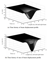
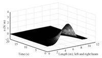
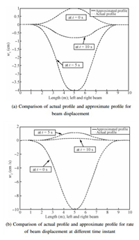
Figs. 4 and 5 show the results of the SNAC controller implementation. It can be observed that the control action is able to bring the beam system to the desired equilibrium state,i.e., both the beam displacement and the rate of the beam displacement go to zero. Analysis of the validity of POD approximation of the underlying PDE system is carried out by comparing the actual state profiles to approximated profiles generated by using (36). Fig. 6 shows that basis functions are able to capture the state profile quite well at the different time instants considered. Note that SNAC controller is developed based on the approximated profile in lumped parameter model. Due to the close approximation,as shown in Fig. 6,control actions calculated from a low-dimensional approximated system are effective in controlling the flexible wing which is a distributed system.
|
Download:
|
| Fig. 4. Time history of state variables. | |
|
Download:
|
| Fig. 5. Time history of continuous control action profile. | |
|
Download:
|
| Fig. 6. Comparison of actual profile and approximate profile. | |
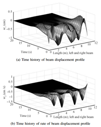
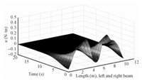
In order to show the versatility of the SNAC approach to initial conditions,state histories from using a different initial condition are provided. These simulation results shown in Figs. 7 and 8 clearly indicate that the system is stabilized. Fig. 7 shows the system trajectories with respect to time. Fig. 8 shows the stabilizing feedback control action which is able to direct the system towards desired equilibrium condition.
|
Download:
|
| Fig. 7. Time histories of beam displacement profile and rate of beam displacement profile. | |
|
Download:
|
| Fig. 8. Time history of continuous control action profile. | |
Next,the need for designing the online adaptive control is shown by simulating the flexible wing motion in the presence of uncertainties. For this purpose,the exact values of a few system parameters were assumed to be unknown which is the equivalent of parametric uncertainties in a system. Furthermore,a bias term is added to the actual system dynamics to make it inherently unstable. The chord length $c$ and lift curve slope $C_{l_\alpha } $ are 1 m and 3 ${\rm rad}^{-1}$ respectively which differ from the actual value listed in Table I. While designing the nominal (offline) control,as discussed in Sections III and IV,10 basis functions are considered,to obtain an approximate lumped parameter model. Same architecture of neural network as before is taken for SNAC and the nominal control is designed. A bias term $\frac{100}{\rho a}w_2 \left( {t,y} \right)$ is added to the right hand side of in the second equation of (34) which is treated as an uncertainty in the controller development. The procedure described in Section 6 is adopted to design an identifier and online adaptive control system.
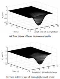
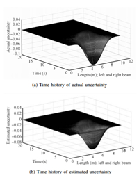
Figs. 9 $\sim$ 11 show the results of the system dynamics with uncertainties. System uncertainty is estimated with a linear-in-parameter neural network. The following basis functions are used to estimate the uncertainty: \begin{align*} &\sigma \left( {w_1 ,w_2 } \right)=[w_1 ,w_2 ,\left( {w_1 } \right)^2,\left( {w_2 } \right)^2,\\ &\quad w_1 w_2 ,\left( {w_1 } \right)^3,\left( {w_2 } \right)^3,\left( {w_1 } \right)^2w_2 ,w_1 \left( {w_2 } \right)^2 ]^{\rm T} \end{align*}
|
Download:
|
| Fig. 9. Time histories of (a) beam displacement profile and (b) rate of beam displacement profile. | |
|
Download:
|
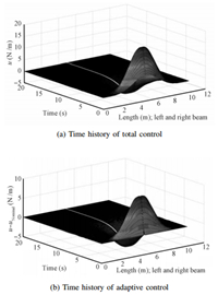
| Fig. 10. Time histories of total control and adaptive control. | |
|
Download:
|
| Fig. 11. Time histories of actual uncertainty and estimated uncertainty. | |
Identifier states and neural network weights are initialized as zero. Fig. 9 shows the system state histories with respect to time under the control action as shown in Fig. 10 (a). Fig. 10 (b) show the extra (adaptive) control needed to compensate for the estimated uncertainty. Fig. 11 (a) and (b) show the actual (modeled) and estimated uncertainties with respect to time, respectively. To see the importance of adaptive control,shown in Fig. 10 (b),the system dynamics was simulated with the nominal (offline) control architecture also.
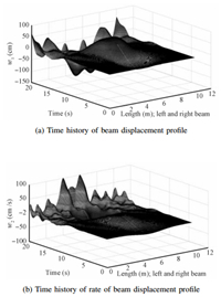
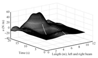
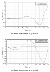
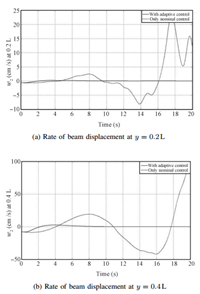
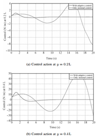
Fig. 12 shows that system is unstable when just the nominal control,designed using SNAC,is applied to the system with uncertainty. Fig. 13 shows the corresponding nominal control action. Figs. 14 $\sim$ 16 compare the results of system trajectory and control action at different spatial points. The control action,which is augmented with adaptive control,stabilizes the system whereas nominal control alone is not sufficient to do so, which clearly shows the need for adaptive control.
|
Download:
|
| Fig. 12. Time histories of beam displacement profile and rate of beam displacement profile. | |
|
Download:
|
| Fig. 13. Time history of continuous control action profile. | |
|
Download:
|
| Fig. 14. Beam displacements at $y$ = 0.2L and $y$ = 0.4L. | |
|
Download:
|
| Fig. 15. Rate of beam displacements at $y$ = 0.2L and $y$= 0.4L. | |
|
Download:
|
| Fig. 16. Control actions at $y=0.2$L and at $y=0.4$L. | |
In this paper,a stabilizing state-feedback control design approach for controlling the heave dynamics of an aircraft$'$s flexible wing problem was developed using reinforcement and adaptive control techniques. The proper orthogonal decomposition technique was used to get a finite dimensional approximate model (lumped parameter model) of a flexible wing by using a set of basis functions. Then,the optimal controller was synthesized using the single-network-adaptive-critic technique for this lumped system. Simulation results show the effectiveness of the designed single-network-adaptive-critic controller for different initial conditions. Further to mitigate the loss in performance due to uncertainties the single-network adaptive critic controller was augmented with a passive identifier based adaptive controller. Numerical results show that under destabilizing uncertainties the single-network adaptive critic controller augmented with adaptive controller is able to stabilize the system. Since the controller development is fairly general,it is possible to extend its applicability to control of other distributed parameter systems under uncertainties.
| [1] | Lasiecka I. Control of systems governed by partial differential equations:a historical perspective. In: Proceedings of the 34th Conference onDecision and Control. New Orleans, LA: IEEE, 1995.2792-2796 |
| [2] | Burns J A, King B B. Optimal sensor location for robust control ofdistributed parameter systems. In: Proceedings of the 1994 Conferenceon Decision and Control. Lake Buena Vista, FL, USA: IEEE, 1994.3967-3972 |
| [3] | Curtain R F, Zwart H J. An introduction to Infinite Dimensional LinearSystems Theory. New York: Springer-Verlag, 1995. |
| [4] | Padhi R, Balakrishnan S N. Optimal dynamic inversion control designfor a class of nonlinear distributed parameter systems with continuousand discrete actuators. The Institute of Engineering and Technology,Control Theory, and Applications, 2007, 1(6): 1662-2671 |
| [5] | Haykin S. Neural Networks. New York: Macmillan College Company,1994. |
| [6] | Gupta S K. Numerical Methods for Engineers. New Delhi: New AgeInternational Ltd., 1995. |
| [7] | Christofides P D. Nonlinear and Robust Control of PDE Systems:Methods and Applications to Transport-Reaction Processes. Boston:Birkhauser Boston Inc., 2001. |
| [8] | Holmes P, Lumley J L, Berkooz G. Turbulence Coherent Structures,Dynamical Systems and Symmetry. Cambridge: Cambridge UniversityPress, 1996.87-154 |
| [9] | Bryson A E, Ho Y C. Applied Optimal Control: Optimization, Estimation,and Control. Washington: Taylor and Francis, 1975 |
| [10] | Lewis F. Applied Optimal Control and Estimation. New Jersey: Prentice-Hall, 1992. |
| [11] | Werbos P J. Neurocontrol and supervised learning: an overview andevaluation. Handbook of Intelligent Control: Neural, Fuzzy and AdaptiveApproaches. New York: Van Nostrand Reinhold, 1992 |
| [12] | Balakrishnan S N, Biega V. Adaptive-critic based neural networks foraircraft optimal control. Journal of Guidance, Control and Dynamics,1996, 19(4): 893-898 |
| [13] | Padhi R, Unnikrishnan N, Wang X, Balakrishnan S N. A single networkadaptive critic (SNAC) architecture for optimal control synthesis for aclass of nonlinear systems. Neural Networks, 2006, 19: 1648-1660 |
| [14] | Padhi R, Balakrishnan S N. Optimal beaver population managementusing reduced-order distributed parameter model and single networkadaptive critics. In: Proceedings of the 2004 American Control Conference.Boston, MA, 2004.1598-1603 |
| [15] | Yadav V, Padhi R, Balakrishnan S N. Robust/optimal temperature profilecontrol of a re-entry vehicle using neural networks. In: Proceedings ofthe 2006 AIAA Atmospheric Flight Mechanics Conference and Exhibit.Keystone, Colorado: AIAA, 2006.21-24 |
| [16] | Prabhat P, Balakrishnan S N, Look D C Jr. Experimental implementationof adaptive-critic based infinite time optimal neurocontrol for aheat diffusion system. In: Proceedings of the 2002 American ControlConference. Alaska, USA: IEEE, 2002.2671-2676 |
| [17] | Chakravarthy A, Evans K A, Evers J. Sensitivity & functional gains fora flexible aircraft-inspired model. In: Proceedings of the 2011 AmericanControl Conference. Baltimore, MD, USA: IEEE, 2010.4893-4898 |
| [18] | Chakravarthy A, Evans K A, Evers J, Kuhn L M. Target tracking strategiesfor a nonlinear, flexible aircraft-inspired model. In: Proceedings ofthe 2011 American Control Conference. San Francisco: IEEE, 2011.1783-1788 |
| [19] | Narendra K S, Annaswamy A M. Stable Adaptive Systems. EnglewoodCliffs, NJ: Prentice-Hall, 1989. |
| [20] | Ioannou P A, Sun J. Robust Adaptive Control. Englewood Cliffs, NJ:Prentice-Hall, 1995. |
| [21] | Böhm M, Demetriou M A, Reich S, Rosen I G. Model reference adaptivecontrol of distributed parameter systems. SIAM Journal of Control andOptimization, 1998, 36(1): 33-81 |
| [22] | Hong K S, Bentsman J. Direct adaptive control of parabolic systems:algorithm synthesis and convergence and stability analysis. IEEE Transactionsof Automatic Control, 1994, 39(10): 2018-2033 |
| [23] | Hong K S, Yang K J, Kang D H. Model reference adaptive control of atime-varying parabolic system.KSME International Journal, 2000, 14(2):168-176 |
| [24] | Krstic M, Smyshlyaev A. Adaptive control of PDEs. Annual Reviews inControl, 2008, 32(2): 149-160 |
| [25] | Demetriou A M, Rosen I G. On-line robust parameter identification forparabolic systems. International Journal of Adaptive Control and SignalProcessing, 15(6): 615-631 |
| [26] | Sirovich L. Turbulence and the dynamics of coherent structures. Quarterlyof Applied Mathematics, 1987, 45(3): 561-590 |
| [27] | Ravindran S S. Proper Orthogonal Decomposition in Optimal Controlof Fluids, NASA/TM-1999-209113. USA, 1999. |
| [28] | Padhi R, Balakrishnan S N. Proper orthogonal decomposition basedoptimal control design of heat equation with discrete actuators usingneural networks. American Control Conference, ACC02-IEEE 1545,2002. |
| [29] | Padhi R, Balakrishnan S N. Proper orthogonal decomposition basedfeedback optimal control synthesis of distributed parameter systemsusing neural networks. In: Proceedings of the 15th American ControlConference. Anchorage, AK: IEEE, 2002.4389-4394 |
| [30] | Ravindran S S. Adaptive reduced-order controllers for a thermal flowsystem using proper orthogonal decomposition. SIAM Journal on ScientificComputing, 2002, 23(6): 1924-1942 |
| [31] | Popov V M. Hyperstability of Control Systems. Berlin: Springer, 1973. |
| [32] | Olver P J. Introduction to Partial Differential Equations. New York:Springer-Verlag, 2013. |
 2014, Vol.1

