Ⅰ. INTRODUCTION

A kind of data-driven control method has been proposed recently^[1],i.e.,the model free adaptive control (MFAC) algorithm which is composed of the dynamic linearization data model (DLDM) and the "control function". Notably,the DLDM does not depend on the concrete mathematical model of the controlled object,which can be calculated based on the output$'$s pseudo gradient at each sample time.

The MFAC was proposed for unknown nonlinear systems,and has been successfully applied to many process control systems^[2]. For the MFAC approach,an equivalent dynamic linearization data model is built at each operation point of the closed-loop system,and then the MFAC controller is designed based on this equivalent data model. Compared with traditional adaptive control methods,no structure information about the plant model is needed during the design of controller and estimator,and no unmodelled dynamics exists. Therefore,the MFAC is suitable for many practical systems since it is robust to system uncertainty.

As one of the data-driven control method,the MFAC has received much attention. For example,most of the MFAC control laws for single-input single output (SISO) systems can be directly extended to complex multi-input multi-output (MIMO) systems^[3]. Inspired by the work of dynamic linearization technique of Hou et al.^[2],a multiple adaptive observer-based control strategy for nonlinear processes is proposed in which the pseudo-partial derivative (PPD) theory is used to dynamically linearize the MIMO nonlinear system^[4].

However,the MFAC is still developing^[5]. The proof of stability and convergence of the tracking problems and parameter tuning are its two open problems. In general,the parameters of MFAC are selected only according to qualitative analysis^[2]. For the same control system,different controller parameters may lead to totally different control results,if we choose the controller parameters according to the stability theorem, carelessly. Especially when working conditions change,the current controller parameters may cause the output response oscillation.

How to get appropriate and robust controller parameters is very important in real application. Although the MFAC is a pure data driven control method which is independent of the process model,it would be helpful to the parameter tuning if the first principle model or identified model is available. Even though it is not an accurate mathematical model,it still can be used to tune the parameters of MFAC to improve the control performance of the closed loop system. The parameter tuning of an improved MFAC without considering noise was discussed preliminarily in [6] where the optimal controller parameters were obtained for several different objective functions by using the approximate identified model. It was shown that the association performance index of square-error and square-input with raise time constraint (which is called Jeu_tr index) makes the system possess better dynamic response,and less iteration times,compared with other indices,such as integral of the squared error (ISE) and integral of the time-weighted absolute error (IAE).

In addition,the external stochastic noise has a great influence on the control system in the industrial filed. Sometime,it is not the Gaussian noise. Generally,the minimized variance of the tracking error can indicate optimization of controller tuning for systems which have Gaussian noise or at least have symmetric probability density functions^[7]. It is still not easy to find the suitable controller parameters during the finite time to guarantee the close-loop system is stable in the high noise environment,due to the limit of modern optimization method. Furthermore,for non-Gaussian systems,the variance of tracking error cannot be used to represent the performance of the closed-loop system alone. The reason is simple: if the interference is non-symmetric,its spread area cannot be purely described by the variance. As a result,a more general measure of uncertainty,namely entropy,should be used to characterize the uncertainty of the tracking error^[8]. This advantage is especially significant in dealing with problems involving non-Gaussian or large Gaussian statistics,where mean square methods may be inadequate. The application of entropy originates from the information theory^[9]. Various types of entropy measures have been introduced to control the stochastic nonlinear system^[10].

In this paper,the parameters tuning problems of dynamic linearization based MFAC are considered. First,the dynamic linearization based MFAC algorithm with control input linearization length constant $L$ = 2 is re-derived using the concept of pseudo gradient proposed in [2]. Then for the unavoidable problem of parameter tuning of stochastic nonlinear system,a minimum entropy performance index is proposed. Combined with the gradient descent technique,the parameter$'$s optimization method is derived. There are a few parameters in the MFAC algorithm,so it is difficult and unnecessary to tune all the parameters at one time. In this paper, the tuning of three key parameters is considered,and a simple offline practical tuning algorithm is given,in which a simplified and approximated model is used. At last,simulation examples for linear and nonlinear systems are given. In the case of Gaussian stochastic noise and non-Gaussian stochastic noise,the dynamic performance of close-loop system based on entropy index tuning parameters has been compared with that of the traditional index, such as ISE and ITAE.

Ⅱ. MODEL FREE ADAPTIVE CONTROL

A general discrete time nonlinear system is given as follows:

\begin{align} y(k + 1) = f(y(k),\cdots ,y(k - m),u(k),\cdots ,u(k - n)), \label{eq1} \end{align}

(1)

where $y(k)$ and $u(k)$ are the system output and input, respectively,$m$ and $n$ are the orders of $y(k)$ and $u(k)$, respectively^[11].

In a traditional model-free adaptive controller,a nonlinear system is transformed into a linear time-varying dynamic system according to the compact format linearization. Then the input and output relationship can be described as follows:

\begin{align} y(k + 1) - y(k) = \varphi (k)[u(k) - u(k - 1)], \end{align}

(2)

where the time-varying parameter $\varphi(k)$ is called pseudo partial derivative. But for some complex systems,the behavior of the current time-varying parameter may become very complex,which leads to the estimation algorithm unable to estimate the dynamic behavior very well in this case. Therefore,a new system input-output relationship is constructed and called partial form dynamic linearization^{[12, 13]}. In the following,the MFAC algorithm is introduced based on partial form dynamic linearization.

At first,assume that system (1) satisfies the generalized Lipschitz conditions^[2],that is

\begin{align} \left| {y({k_1} + 1){\rm{ - }}y({k_2} + 1)} \right| \le b\left| {{u_L}({k_1}) - {u_L}({k_2})} \right|, \end{align}

(3)

for $u_L(k_1)\neq u_L(k_2)$ and any $k_1\neq k_2$,$k_1$,$k_2\geq 0$,where $u_L(k)=[u(k)\ u(k-1)]^{\rm T}$,$b$ is a positive constant.

When the nonlinear system (1) satisfies the above conditions, bounded $\phi_1(k)$ and $\phi_2(k)$ must exist such that system (1) can be denoted as the following partial form dynamic linearization (PFDL) data model:

\begin{align} \begin{split} y(k + 1)& - y(k) = {\varphi _1}(k)[u(k) - u(k - 1)]+\\ &{\varphi _2}(k)[u(k - 1) - u(k - 2)], \end{split} \label{eq4} \end{align}

(4)

for any time $k$,which can be shortened to

\begin{align} \Delta y(k + 1) = {\varphi _1}(k)\Delta u(k) + {\varphi _2}(k)\Delta u(k - 1). \end{align}

(5)

It is well known that the system output at the current time is always affected by the system inputs at the current time and previous time. Therefore,(4) or (5) represents more input information about the controlled plant than (2).

An expanded integrated square error index (6) is used to solve the reference trajectory tracking problem.

\begin{align} J(u(k)) = {[{y^*}(k + 1) - y(k + 1)]^2} + \lambda {[u(k) - u(k - 1)]^2}, \end{align}

(6)

where $\lambda$ is the weighting factor. In this criterion function,the first part $[y^{*}(k+1)-y(k+1)]^2$ can reduce the steady tracking error and restrain noise,whereas the second part $[u(k)-u(k-1)]^2$ can restrict a great change in the control input.

According to gradient descent technique,the control law is

\begin{align} \begin{split} u(k) &= u(k - 1)+\\ & \frac{{{\rho _1}{\varphi _1}(k)[{y^*}(k + 1) - y(k)]}}{{\lambda + \varphi _{_1}^2(k)}} - \frac{{{\rho _2}{\varphi _1}(k){\varphi _2}(k)\Delta u(k - 1)}}{{\lambda + \varphi _{_1}^2(k)}}, \end{split} \label{eq7} \end{align}

(7)

where $\rho_k(0 < \rho_k < 2)$,$k$ = 1,2 is optimal step factors. The second order pseudo partial derivatives $\varphi_1(k)$ and $\varphi_2(k)$ can be estimated according the criterion function

\begin{align} \begin{split} &J({\varphi _1}(k),{\varphi _2}(k))= [y(k) - y(k - 1) - {\varphi _1}(k)\Delta u(k - 1)+\\ &\quad {\mu _1}{[{\varphi _1}(k) - {\hat{\varphi}_1}(k - 1)]^2}+ {\mu _2}{[{\varphi _2}(k) - {\hat{\varphi} _2 }(k - 1)]^2}, \end{split} \label{eq8} \end{align}

(8)

where $y(k)$ is the $k$-th output value,and $\mu_k$,$k=1,2$ is the given weighting factor. And the pseudo partial derivatives are

\begin{align} &{{\hat \varphi }_1}(k)= {{\hat \varphi }_1}(k - 1)+ \frac{{{\eta _1}\Delta u(k - 1)}}{{{\mu _1} + \Delta {u^2}(k - 1)}}\times\notag\\ &\quad [\Delta y(k) - {{\hat \varphi }_1}(k - 1)\Delta u(k - 1) - {{\hat \varphi }_2}(k - 1)\Delta u(k - 2)],\\ \end{align}

(9)

\begin{align} &{{\hat \varphi }_2}(k) = {{\hat \varphi }_2}(k - 1)+ \frac{{{\eta _2}\Delta u(k - 2)}}{{{\mu _2} + \Delta {u^2}(k - 2)}}\times\notag\\ &\quad [\Delta y(k) - {{\hat \varphi }_2}(k - 1)\Delta u(k - 2) - {{\hat \varphi }_1}(k - 1)\Delta u(k - 1)], \label{eq10} \end{align}

(10)

where $\eta_1$ and $\eta_2$ are appropriate step factors.

As shown in the control law (7),(9) and (10),this kind of controller has nothing to do with the model structure or the order of the system. It is designed only by the input and output data.

Ⅲ. PARAMETERS TUNING BASED ON MINIMUM ENTROPY OPTIMIZATION

The research about parameter tuning of the MFAC is of great significance to the applications of MFAC in practice engineering. There are a few parameters that need to be tuned for the MFAC (7), (9),and (10),and the suitable parameters are not easy to be obtained.

Firstly,the adjustable parameters of a second order partial format adaptive controller are $\rho_1$,$\rho_2$,$\lambda$ , $\eta_1$,$\eta_2$,$\mu_1$ and $\mu_2$. After a lot of engineering practices and simulation experiments,it is found that the key parameters are $\lambda$,$\rho_1$,and $\rho_2$. Parameter $\rho_2$ just appears in the second order partial format. Generally,the range of $\rho_2$ is (0,2) and $\lambda$ can be determined according to [2]. When $\rho_2/ \rho_1$ is constant and an appropriate $\lambda$ given,$\rho_1$ will be the exclusive parameter that should be tuned.

A. General Noise Case

Since the stochastic noise exists in the unknown plant (1),a minimum entropy index is proposed. Entropy is a unified probabilistic measure of uncertainty quantification. The entropy of a continuous type random error variable $x$ is defined as^[14]

\begin{align} H(x) = - \int\nolimits_{ - \infty }^\infty {\gamma (x)} \ln \gamma (x){\rm d}x,\label{eq11} \end{align}

(11)

where $\gamma(x)$ is the probability density function of $x$. The integration extends only over the region where $\gamma(x)\neq 0$^[15]. Here,the entropy index can measure the dispersion of a stochastic process rather than its mean or variance,so it provides a general description of stochastic systems without constraints of certain distributions. This advantage is especially significant in dealing with non-Gaussian statistics problems,when mean-square methods may be inadequate.

The MFAC is an effective approach for actual systems without accurate model information,and the control effect is determined by control parameters. Generally,we can select appropriate parameters according to engineering experience or a trail and error method. Reference [2] gives a general parameter rule and stable parameter domain. But the system model information,if available,would be helpful for obtaining quantitative parameter descriptions for an endless variety of processes. This is the same as the PID parameter tuning,such as Z-N,ISE and ITAE indices,even though PID is the most classical data-driven controller. That means controller design and parameter tuning are two different problems,and the model information is also necessary for the quantitatively parameter tuning problem of model-free controller. Here we suppose that system model is known or identified from actual process data. The model for parameter tuning may be not as accurate as what we need for controller design.

Assume that the approximate or identified system model can be represented by the following nonlinear ARMAX equation:

\begin{align} \begin{split} y(k + 1) = f(y(k),\cdots ,y(k - m),\\ u(k),\cdots ,u(k - n),\omega (k)), \end{split} \label{eq12} \end{align}

(12)

where $y(k)$ is the measured output from the system,$u(k)$ is the controller output,$\omega(k)$ is the bounded random disturbance which has an assumed known probability density function $\gamma_{\omega(k)}$,$\omega(k)\in [a,b]$.

The output tracking error is defined as

\begin{align} \begin{split} &e(k) = y(k) - {y^*}(k)=\\ &\quad f(y(k - 1),\cdots ,y(k - m),\\ &\quad u(k),\cdots u(k - n),\omega (k)) - {y^*}(k):=\\ &\quad g(y(k - 1),\cdots ,y(k - m),\\ &\quad u(k),\cdots ,u(k - n),\omega (k),{y^*}(k)), \end{split} \label{eq13} \end{align}

(13)

where $y^*(k)$ is the reference trajectory and $g(\cdot)$ is a nonlinear function of reference trajectory $y^*(k)$ and system measured input and output. Denote all known information vectors at time $k$ as

\begin{align} &\eta (k) = \notag\\ &\quad (y(k - 1),\cdots ,y(k - m),u(k - 1) \cdots u(k - n),{y^*}(k)), \end{align}

(14)

then (13) can be further expressed as

\begin{align} e(k) = g(\eta (k),u(k),\omega (k)). \end{align}

(15)

Obviously,(15) is a general form of the tracking error. Since $g(\cdot)$ is a bounded function and $\omega(k)$ is defined on $a,b$,$e(k)$ will also be bounded if $u(k)$ is bounded. The tracking error $e(k)$ is not necessarily Gaussian distribution because $\omega(k)$ is a general stochastic noise. Therefore,it is not appropriate to simply use variance to characterize its randomness. Here entropy is employed to represent the uncertainty of the tracking error. In this case,the probability density functions of $e(k)$ should be first established.

Using the probability theory^[8],the probability density functions of $e(k)$ can be formulated as

\begin{align} \begin{split} {\gamma _{e(k)}}(\eta (k),u(k),x) = {\gamma _\omega }({g^{ - 1}}(\eta (k),u(k),x))\times\\ \quad \frac{{{\rm d}({g^{ - 1}}(\eta (k),u(k),x))}}{{{\rm d}x}},x \in [{a_e},{b_e}], \end{split} \label{eq16} \end{align}

(16)

where the variable symbol $x$ denotes the tracking error,i.e., $x=e(k)$,and $g^{-1}(\cdot)$ is the inverse function of $g(\cdot)$ with respect to $\omega(k)$,$a_e$ and $b_e$ are upper and lower bounds obtained from the tracking error (13). In this case,$\gamma_{e(k)}(\cdot )$ is continuous and first order differentiable with all its variables.

It can be seen from (16) that the shape of the probability density functions of the tracking error at time $k$ is determined by the controller output $u(k)$. Generally,the controller design should be performed such that the probability density function of the tracking error is as narrow as possible. This is simply because a narrow distribution function generally indicates that the uncertainty of the related random variable is small,which also corresponds to a small entropy value. According to the analysis of the above paragraph,parameter $\rho_1$ has a great effect on the controller output $u(k)$. For this purpose,the performance function (11) is re-written as

\begin{align} J({\rho_1},&{\rho _2},\lambda ) = - \int\nolimits_0^N {\int\nolimits_{a_e}^{b_e} {{\gamma _{e(k)}}(\eta (k),u(k),x)}}\times\notag\\ &\ln {\gamma _{e(k)}}(\eta (k),u(k),x){\rm d}x{\rm d}t, \end{align}

(17)

where $N$ is the control period.

The performance function is a general nonlinear function with respect to $\rho_{1},\rho_2,\lambda$. Sometimes it is not necessarily convex. Therefore,the tuning of parameter $\rho_1$ is a nonlinear optimization problem that can be solved using the following gradient algorithm:

\begin{align} {\rho _1}(i + 1) = {\rho _1}(i) - b \frac{{\partial J}}{{\partial {\rho _1}(i)}}, \end{align}

(18)

where $i$ is current iteration number of the optimizing. Generally,the optimization algorithm (17) can only guarantee the search for a local minimum. According to (17),we have

\begin{align} \begin{split} \frac{{\partial J}}{{\partial {\rho _1}}} = - \int\nolimits_0^N {\int\nolimits_{a_e}^{b_e} {\frac{{\partial {\gamma _{e(k)}}(\eta (k),u(k),x)}}{{\partial {\rho _1}}}} }\times\\ \quad (\ln {\gamma _{e(k)}}(\eta (k),u(k),x) + 1){\rm d}x{\rm d}t \end{split} \label{eq19} \end{align}

(19)

Here we just give the tuning of parameters $\rho_1$. The tuning of parameter $\lambda$ and $\rho_2$ is similar. Actually,the performance function (17) is a function of parameters $\lambda$, $\rho_1$ and $\rho_2$. Using the gradient algorithm,we can get the optimal values of $\lambda$ and $\rho_2$. \begin{align*} {\rho _2}(i + 1) = {\rho _2}(i) - c \frac{{\partial J}}{{\partial {\rho _2}(i)}}, \end{align*} \begin{align*} \lambda (i + 1) = \lambda (i) - d \frac{{\partial J}}{{\partial \lambda (i)}}, \end{align*} with \begin{align*} \begin{split} \frac{{\partial J}}{{\partial {\rho _2}}} = - \int\nolimits_0^N {\int\nolimits_{a_e}^{b_e} {\frac{{\partial {\gamma _{e(k)}}(\eta (k),u(k),x)}}{{\partial {\rho _2}}}} }\times\\ \quad (\ln {\gamma _{e(k)}}(\eta (k),u(k),x) + 1){\rm d}x{\rm d}t, \end{split} \end{align*} \begin{align*} \begin{split} \frac{{\partial J}}{{\partial \lambda }} = - \int\nolimits_0^N {\int\nolimits_{a_e}^{b_e} {\frac{{\partial {\gamma _{e(k)}}(\eta (k),u(k),x)}}{{\partial \lambda }}} }\times\\ \quad (\ln {\gamma _{e(k)}}(\eta (k),u(k),x) + 1){\rm d}x{\rm d}t. \end{split} \end{align*}

B. Linear Gaussian Case

The Gaussian stochastic noise is a special case of general stochastic noise. It has symmetrical probability density,and the parameter is optimal when the error is the smallest value. The expression of the minimum entropy optimization algorithm is re-derived by the probability density of Gaussian stochastic noise.

Consider the following CARMAX model widely used in stochastic and adaptive control:

\begin{align} y(k) = \sum\limits_{j = 1}^m {{a_j}y(k - j)} + \sum\limits_{l = 0}^n {{b_l}u(k - l) + \omega (k)}, \end{align}

(20)

where the stochastic noise $\omega(k)$ is Gaussian distribution whose probability density function is

\begin{align} {\gamma _\omega }(x) = \frac{1}{{\sqrt {2\pi } \sigma }}{{\rm e}^{ - \frac{{(x - \mu )}^2}{2{\sigma ^2}}}},x \in ( - \infty ,+ \infty ). \end{align}

(21)

This system is a special case of the general system (12) and its tracking error takes the following simple form:

\begin{align} \begin{split} e(k) &= y(k) - {y^*}(k)= \sum\limits_{j = 1}^m {{a_j}y(k - j)} +\\ & \sum\limits_{l = 1}^n {{b_l}u(k - l) + {b_0}u(k) + \omega (k) - {y^*}(k)}. \end{split} \label{eq22} \end{align}

(22)

Accordingly,the known vector $\eta(k)$ in (15) is grouped by

\begin{align} \eta (k) = \sum\limits_{j = 1}^m {{a_j}y(k - j)} + \sum\limits_{l = 1}^n {{b_l}u(k - l){\rm{ - }}{y^{\rm{*}}}(k)}. \end{align}

(23)

This leads to a linear tracking error given by

\begin{align} \begin{split} e(k) &= \eta (k) + {b_0}u(k) + \omega (k):=\\ & g(\eta (k),u(k),\omega (k)). \end{split} \label{eq24} \end{align}

(24)

Then we have

\begin{align} \begin{split} \omega(k)&= e(k){\rm{ - }}\eta (k) - {b_0}u(k)=\\ & {g^{ - 1}}(\eta (k),u(k),x), \end{split} \label{eq25} \end{align}

(25)

here the variable symbol $x$ denotes the tracking error,i.e.,$x = e(k)$. Then after substituting the inverse function $g^{-1}(\cdot)$ into (16),the probability density functions of the tracking error can be formulated as follows:

\begin{align} {\gamma _{e(k)}}(\eta (k),u(k),x) = \frac{1}{{\sqrt {2\pi } \sigma }}{{\rm e}^{ - \frac{{(x - \eta (k) - {b_0}u(k) - \mu )}^2}{2{\sigma ^2}}}}. \end{align}

(26)

Therefore,

\begin{align} &\frac{{\partial {\gamma _{e(k)}}(\eta (k),u(k),x)}}{{\partial {\rho _1}(i)}} = \frac{{\partial {\gamma _{e(k)}}(\eta (k),u(k),x)}}{{\partial u(k)}}\times \frac{{\partial u(k)}}{{\partial {\rho _1}(i)}},\notag\\ &\frac{{\partial {\gamma _{e(k)}}}}{{\partial u}} = \frac{{{b_0}}}{{2{\sigma ^3}\sqrt {2\pi } }} {{\rm e}^{ - \frac{{(x - \eta (k) - {b_0}u(k) - \mu )}^2}{2{\sigma ^2}}}}, \label{eq27} \end{align}

(27)

\begin{align} \begin{split} &\ln {\gamma _{e(k)}}(\eta (k),u(k),x)=\\ &\quad \ln \frac{1}{{\sqrt {2\pi } \sigma }} - \frac{1}{{2{\sigma ^2}}}{(x - \eta (k) - {b_0}u(k) - \mu )^2}. \end{split} \label{eq28} \end{align}

(28)

According to (7),we have \begin{align*} \frac{{\partial u(k)}}{{\partial {\rho _1}}} = \frac{{{\varphi _1}(k)[{y^*}(k + 1) - y(k)]}}{{\lambda + \varphi _{_1}^2(k)}}. \end{align*} Then simultaneously considering (19),(27) and (28),the Gaussian-entropy optimization equation is

\begin{align} \begin{split} \frac{{\partial J}}{{\partial {\rho _1}}} &= - \int\nolimits_0^N {\int\nolimits_{{a_e}}^{{b_e}} {\frac{{{b_0}}}{{{\sigma ^3}\sqrt {2\pi } }} {{\rm e}^{ - \frac{{(x - \eta (k) - {b_0}u(k) - \mu )}^2}{2{\sigma ^2}}}}}} \times\\ &\frac{{{\varphi _1}(k)[{y^*}(k + 1) - y(k)]}}{{\lambda + \varphi _{_1}^2(k)}} \times\\ &\left(\ln \frac{1}{{\sqrt {2\pi } \sigma }} - \frac{1}{{2{\sigma ^2}}}{(x - \eta (k) - {b_0}u(k) - \mu )^2} + 1\right){\rm d}x{\rm d}t \end{split} \label{eq29} \end{align}

(29)

C. Practical Tuning Algorithm

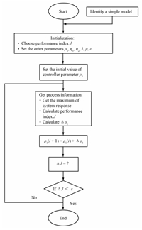
The parameter tuning process of dynamic linearization based MFAC is shown in the following:

1) Identify a simple model for system (12) or (20) according to off-line data,which can be not very accurate.

2) Select an appropriate performance index $J$ in (17) according to the control requirement.

3) Initialize other parameters,such as $b$,$\rho_2$,$\lambda$, $\eta_1$,$\eta_2$,$\mu_1$ and $\mu_2$.

4) Give an initial parameter $\rho_1$ in the range of (0,2).

5) Compute the gradient function of $J$ with respect to parameter $\rho_1(i)$,that is,$\frac{\partial J}{\partial {\rho _1}}(i)$.

6) Update the tuning parameter $\rho_{1}$ according to \begin{align*} {\rho _1}(i + 1) = {\rho _1}(i) + \Delta {\rho _i}, \end{align*} where $\Delta {\rho _1} = - b \cdot \frac{\partial J}{\partial {\rho _1}(i)}$.

7) If the change of index $J$ meets $\Delta J < \varepsilon $,the parameter tuning is over; else jump to step 5) and keep tuning.

The procedure of tuning is shown in Fig. 1.

Ⅳ. SIMULATION STUDY

In this section,two different systems are used to test the availability and effectiveness of the proposed entropy tuning method. They are a third-order linear system with large delay and a time-varying nonlinear system. In order to analyze the effectiveness of the minimum entropy parameter tuning method under random noise,the other two classic performance indexes are given for comparison. The optimum PID controller algorithm was introduced by [16]. And the more general index is

\begin{align} J = {\int_0^\infty {\left[{{t^n}e(t)} \right]} ^2}{\rm d}t, \label{eq30} \end{align}

(30)

where $e(t)$ is the error signal of the controller. When $n$ = 0,$J$ is known as the ISE criterion^[17].

In the parameter optimization,ITAE is often used as the performance index^[18],and it is described as

\begin{align} J = \int_0^\infty {t|e(t)|} {\rm d}t. \end{align}

(31)

For the Gaussian and non-Gaussian stochastic noise,the parameter of MFAC (7),(9),(10) is optimized by three performance indices, i.e.,ISE,ITAE,and minimum entropy index.

A. Example of Linear System with Large Delay

Given a third-order large inertial delay system^[19]:

\begin{align} G(s) = \frac{{K{{\rm e}^{ - \tau s}}}}{{{{\left( {1 + Ts} \right)}^3}}}, \end{align}

(32)

where $K$ = 5,$T$ = 3,$\tau$ = 60.

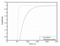
In engineering practice,it is common that any higher order and complex objectives can be approximated by a second-order inertial model plus time delay. Suppose that the first principle model and the identified model are available as shown by (32) and (33), respectively. We can see from Fig. 2 that it is not an accurate mathematical model. In the following,we will show that it still can be used to tune the parameters of MFAC to improve the control performance of the closed loop system. The result of parameter tuning is accepted even the model identification error is very large.

Suppose that the approximate model is

\begin{align} G(s) = \frac{{K{{\rm e}^{ - \tau s}}}}{{{{\left( {1 + Ts} \right)}^2}}}, \end{align}

(33)

where $K$ = 5,$T$ = 2,$\tau $ = 50. It is shown in Fig. 2 that the simple approximate model has the same stable gain but a totally different dynamic response. In this simulation,other parameters are given: $\rho_2$ = 0.35,$\lambda$ = 1,$\eta_1$ = 1,$\eta_2$ = 1,$\mu_1$ = 1 and $\mu_2$ = 2.

Parameter Optimization Effect on the System Stability

i) The case of Gaussian stochastic noise

During the simulation experiment,50 groups of 2.5 % Gaussian stochastic noise are arbitrarily selected. The probability distribution of the Gaussian stochastic noise refers to (21). In order to test and verify the effectiveness of different parameter optimization criteria,every performance index is implemented under the same disturbance.

After 50 groups of Gaussian stochastic noise disturbance experiments,50 groups of different parameter $p_1$ are got. First,it is considered whether the step output response of close-loop system (32) and (7) with the tuned parameter is stable or not. The results are listed in Table I.

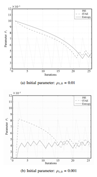
As shown in Table I,the number of stable responses under the minimum entropy index is the highest. From the tuning result,we know the optimal parameter is near 0.003,so the initial values $\rho_{1,0}$ = 0.01 and 0.001 represent the two different optimizing directions. It is shown that 50 groups parameter obtained from entropy criterion are all appropriate and can get stable responses even if the optimization is from a different direction. Whereas the results obtained from the traditional indexes,such as ISE and ITAE,are not encouraging. It seems that these two criterions are not very adaptive to the big noise situation. The reason is obvious that the existing stochastic noise is considered in designing of minimum entropy optimization but not in ISE and ITAE methods. Controller parameter is optimized according to the effect degree of stochastic noise,therefore,the minimum entropy algorithm can guarantee the controlled system stable under any Gaussian stochastic noise.

ii) The case of non-Gaussian stochastic noise

Suppose that the probability distribution of the non-Gaussian stochastic noise is

\begin{align} \gamma (x) = \left\{ {\begin{array}{*{20}{lll}} \frac{3}{{4\sqrt 5 }}(1 - 0.2{x^2}),&\left| x \right| \le \sqrt 5 ,\\ 0,&{\rm otherwise}. \end{array}} \right. \label{eq34} \end{align}

(34)

Similar to the Gaussian noise experiment (1),50 groups of 2.5 % non-Gaussian stochastic noise are arbitrarily selected. The closed system stability is considered,in which the optimal controller parameters are calculated from three different performance index, i.e.,ISE,ITAE,and entropy index,respectively. After 50 groups of non-Gaussian stochastic noise disturbance experiments,the numbers of stable responses are listed in Tables II and III. Here the stable ratio is defined as

\begin{align} \eta = \frac{\mbox{number of stable response}}{\mbox{total test number}}. \end{align}

(35)

As shown in Table II,the result of stability simulation is similar to the Gaussian noise case. The results obtained from the traditional indexes,such as ISE and ITAE,are worse than those of the entropy indexes. It is noted that in the non-Gaussian noise experiment,the stable degrees of ISE and ITAE drop down significantly,while the stable degree of the entropy is the same as the Gaussian noise experiment. The minimum entropy index has better performance in the case of Gaussian and non-Gaussian noise.

It can be shown from Table III that the stable ratio of non-Gaussian noise is much bigger than that of Gaussian noise for traditional indices ISE and ITAE. Furthermore,the traditional performance index cannot completely satisfy the stability requirement under the non-Gaussian stochastic noise circumstance. However,the minimum entropy tuning algorithm can guarantee the system stable in the both cases of Gaussian and non-Gaussian noise.

In order to ensure the controlled system is stable under different performance indices,the stochastic noise is decreased as 1 %. The parameter $\rho_1$ tuning process from the two directions ($\rho_{1,0}$ = 0.01 or $\rho_{1,0}$ = 0.001) are shown in Fig. 3. Fig. 4 shows the performance index changing with iterations. Relatively,the entropy method has a more rapid convergence rate and more stable optimal results than those of the ITAE and ISE indices.

1) Control Results Under Different Performance Index Parameter Optimization

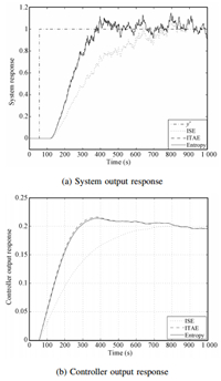
In the case of the non-Gaussian stochastic noise ($\pm1$ %),the initial parameters are $\rho_{1,0}$ = 0.01,$\rho_{1,0}$ = 0.001, the parameter $\rho_{1}$ of the dynamic linearization MFAC is tuned using ISE,ITAE,and minimum entropy optimization indices, respectively. The system output respond and controller output under different performance indexes are shown in Figs. 5 and 6. Even under the conditions that system noise is small and the ISE or ITAE method can obtain desired parameters,the control response under the entropy index is very good,which has more rapid response than that of ISE index. The dynamic response results of three performance indices are listed in Table IV.

As shown in Table IV,the dynamic response of ISE is too slow in the case of the non-Gaussian noise. Besides,the overshoot of the ISE method is still very large. The results of the ITAE and entropy are approximate. But in the view of the rising time, entropy has a better response speed. Therefore,minimum entropy makes the system have a better dynamic performance,which has the less rising time,the less setting time,the smaller overshoot value and so on.

The following experiment is designed to change the system parameter of the controlled objective in order to test the robustness of controller parameter tuned by ISE,ITAE and Entropy methods,respectively. Here the system parameters are changed as follows: \begin{align*} \left\{ {\begin{array}{*{20}{l}} {K = 5,T = 3,\tau = 60,0 < t \le 1 500}\\ {K = 4.5,T = 0.8,\tau = 50,1 500 < t \le 3 000}\\ {K = 5,T = 3,\tau = 60,3 000 < t \le 4 500} \end{array}} \right. \end{align*}

At the time of $1 500 < t < 3 000$, system parameters,such as open-loop gain $K$,time constant $T$ and delay time all change. The system step response and controller output are given in Fig. 7,in which controller parameters are selected as the same as Table IV. It is shown that system responses are not affected by the changing of system. That means the entropy method has good robustness.

B. Example of Time-varying Nonlinear System

The similar experiment is designed to verify the robustness and dynamic stability of a nonlinear system. Three parameter optimization indices,ISE,ITAE and entropy are compared.

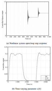
Given a nonlinear system,which consists of two nonlinear subsystems^[20] \begin{align*} &y(k + 1) =\\[-2mm] &\quad \left\{ {\begin{array}{*{20}{lllll}} \frac{{y(k)}}{{1 + y{{(k)}^2}}} + u{{(k)}^3},&k \le 500,\\ \frac{{y(k)y(k - 1)y(k - 2)u(k - 1)(y(k - 2) - 1) + a(k)u(k)}}{{1 + y{{(k - 1)}^2} + y{{(k - 2)}^2}}},&k > 500, \end{array}} \right. \end{align*} where $a(k)=1+{\rm round}(k/500)$,the second subsystem has a step time-varying parameter $a(k)$. Therefore,the structure,order and parameter of this system are time-varying. The open-loop step response of the nonlinear system (35) is shown in Fig. 8 (a). Fig. 8 (b) is the change process of the time-varying parameter $a(k)$. It is shown that the open-loop response has great oscillation at 500 s and 750 s,and the steady output value changes with time. That is because the structure of controlled objects and time-varying parameter $a(k)$ change with time. Here the approximate model (33) is still used for controller parameter tuning.

In the case of the non-Gaussian stochastic noise ($\pm$ 4 %), the initial parameter is $\rho_{1,0}$ = 0.8. Parameter $ \rho_{1}$ is tuned using ISE,ITAE and minimum entropy optimization methods,respectively. Here given other parameters are $\lambda$ = 2,$\rho_2$ = 0.35,$\eta_1$ = 1,$\eta_2$ = 1, $\mu_1$ = 1 and $\mu_2$ = 2.

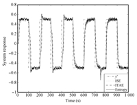
After tuning by ISE,ITEA,and entropy indices,we selected optimal parameters as $\rho_1$ = 0.16888 (ISE),$\rho_1$ = 0.19897 (ITAE),$\rho_1$ = 0.27689 (entropy). The close-loop system responses under different parameters are given in Fig. 9. The controlled object is the first subsystem at the time of $0\leq t\leq 500$,in which time-varying parameter $a(k$) has no influence on it. Then its output response is rapidly tracking the set-point $y^{\ast}$. However,at the time of $500\leq t\leq 1 000$,the controlled object is the second subsystem. Therefore, the system output is affected by time-varying parameter changing at 750 s. Even the structure,order and parameter of the controlled object are time-varying,the close-loop system response obtained by the entropy index shows stronger robustness,rapid convergence rate and accurate tracing result.

Ⅴ. CONCLUSION

The MFAC method is considered,in which the system input and output relationships are described as the partial form linearization data model. Then the minimum entropy idea is used to solve the parameter optimization problem of the MFAC in the case of Gaussian noise and non-Gaussian noise. According to the probability distribution of stochastic noise,the entropy recursive optimization algorithm is derived in the case of general random noise. By choosing a lot of Gaussian stochastic noise and non-Gaussian stochastic noise,the universality of minimum entropy optimization algorithm is verified. In comparison with the other traditional performance indices,such as ISE and ITAE,it is found that: the existing stochastic noise has been considered in the designing of minimum entropy index,so the entropy optimization algorithm can guarantee the controlled system stable under Gaussian or non-Gaussian stochastic noise. Meanwhile the optimal parameter obtained from the minimum entropy index can assure that the system has better dynamic performance,such as less rising time,less stability time and smaller overshoot.