BATCH and semi-batch reactors are widely used in chemical industry for high value added products because of their flexibility. Batch process has more complicated and higher nonlinear mechanism than continuous process. Exothermic chemical reaction generally occurs in these reactors,in which the batch process can be split into heat-up and subsequent reaction stages. Both heat-up and reaction stage require strict temperature control in this kind of reaction. The staged temperature control problem has been described by Chylla and Haase[1, 2]. The temperature control problem of Chylla-Hasse reactor is usually considered as benchmark to test control algorithm because of its complex reaction mechanism,violent heat-releasing,product variety and other features.
The control task of the Chylla-Hasse benchmark contains two aspects: the reactor temperature accurately tracks the reference temperature trajectory in the heat-up period,and the temperature is controlled exactly at the given value during the reaction stage,i.e.,the temperature deviation is not more than $\pm~0.6$ K. There are many uncertain factors that should be considered,such as environment temperature,heat transfer coefficient changing with batch and the raw material concentration varying,which all require the controller to have stronger robustness.
Traditional cascade PID control is widely used to control the reactor temperature in practical industry,in which the reactor temperature is the master and the cooling jacket temperature is a slave. This kind of control method is very simple and convenient, but the control performance is not satisfying for some strict requirement,especially for the high precision temperature control of the Chylla-Hasse reactor.
Therefore,various new control methods were presented to solve the Chylla-Hasse benchmark problem in the literatures. The model predictive control concept combined with extended Kalman filter was proposed in [3]. The extended Kalman filter is used to built the prediction model of reaction heat and heat transfer coefficient in order to estimate these parameters online,then nonlinear model predictive control is introduced to control reactor temperature according to these estimations. Another nonlinear adaptive control was introduced to solve the Chylla-Hasse benchmark in [4],where the nonlinear adaptive controller is the master controller to adjust the desired trajectory for the underlying PI controller. A feed-forward control strategy with extended Kalman filter was proposed for the high-precision tracking problem in [5]. The feed-forward signal is calculated by the inverse model of batch process,and the Kalman filter is also used to estimate the reaction heat and heat transfer coefficient online. Because of the precise process model and parameter estimations,this feed-forward and feedback hybrid control can guarantee the tracking error to be small. A self-tuning regulator with parameter estimation was proposed in [6],where the unscented Kalman filter is adopted to estimate uncertain parameters of system model without delay and calculate the desired temperature trajectory for the cooling jacket. A novel sensitivity compensating nonlinear control approach within generic model control framework for processes exhibiting input sensitivity was proposed in [7]. The approach defined a new process,new control and set point to drive original process to its desired point. In [8],a simple and efficient control scheme was given for the time optimal operation of exothermic semi-batch reactors.
It is shown from these works that the main control method for Chylla-Hasse benchmark is combined with the parameter estimation and mathematical modeling,which needs the total information of reactor mechanism and vast online calculation. However,the accurate mathematical model of batch process is hard to be obtained in practice because of the complex and incomplete known reactor mechanism,and the vast calculation online is hard in real industry because of the limit of hardware condition.
Recently,iterative learning control (ILC)[9] has been proposed and applied to many batch or repetitive processes. The control performance of the repetitive system which executes the same task multiple times can be improved by learning from previous executions (trials,iterations,passes). With the development of ILC theory, ILC has two main control structures: open-loop,closed-loop and various learning laws: PID-type,high-order and optimal learning law[10].
However,the traditional iterative learning control requires that the controlled process must satisfy some strict conditions,such as the initial states of each batch process must be totally the same; the process model and the reference trajectory are also the same in each batch[11]. But these strict constraints are usually unsatisfied in practice. For example,there are some obvious difference in each Chylla-Hasse batch. Firstly,impurity and quality conditions of monomer in the reactor is random,so the initial states of the process is random. Secondly,uncleaned high viscous polymer is attached on the inner wall of the reactor, which results in the heat transfer coefficient varying with both iterative (batch to batch) and time (in one batch) axes. It means that the process model is time-varying and batch-varying. So the traditional ILC is not suitable for the Chylla-Hasse problem.
Many new adaptive ILC algorithms have been proposed to solve the above bottleneck problem,which can be classified into two categories. One is that the ILC algorithm is combined with some identification procedures in time domain or iterative domain,such as the identification of process model,system parameters or controller parameters. A hybrid method of iterative learning control and recursion least squares (RLS) was proposed in [12] to solve the problem of random initial condition and random reference trajectory. Here RLS is used to modify the learning rate of controller adaptively. The open-loop and close-loop P-type iterative learning control were proposed to overcome the sensor saturation in [13]. The combination of time-domain and iterative-domain identification was developed in [14]. In [15],a varying-order learning algorithm was proposed for enhancing tracking performance against repositioning errors. The iterative-domain identification can make up the drawback of time-domain identification,which is effective in some systems containing uncertain parameters. Reference [16] introduce the Kalman filter into ILC control,where the Kalman filter is used to estimate system parameters. Then iterative control law is optimally solved according to linear quadric optimal index. In [17],the iterative learning control was considered for a class of linear discrete-time switched systems with arbitrary switching signals. The first order P-type ILC scheme can be used to achieve perfect tracking over the whole time interval. A model reference adaptive control strategy in [18] was used to design ILC controller for a class of repeatable nonlinear systems with uncertain parameters, high relative degree,initial output resetting error,input disturbance and output noise.
The second category of adaptive ILC is the application of Lyapunov method. Lyapunov method provides an effective way to solve the control problem of non-linear process. It also can be used in iterative learning control system to solve the adaptive problem. Iterative learning control is considered as an adaptive problem which was solved by Lyapunov theory in [19]. A composite Lyapunov function is given in [20],which includes significant system information in both time and repetition learning horizons. The composite function is an addition of traditional Lyapunov function and an norm of parametric learning errors which reflects the variation of system status.
In addition,iterative learning control provides a good framework for batch or repetitive system. Many outstanding control techniques can be used under this standard framework. Reference [21] provides a kind of ILC method with feedforward-feedback structure. The feedback part is PID controller which is used to keep system stable,and the feedforward part is iterative learning control, which aims at tracking reference trajectory and adjusting PID parameters. Neural network and minimum entropy strategy were combined with the adaptive iterative learning control in [22]. In [23],by representing an iterative learning control system as a two-dimensional system and using the philosophy of model predictive control and performance model reference control,a two-dimensional performance model based model predictive iterative learning control scheme is proposed. These adaptive ILC algorithms generally need some mathematic assumptions and relative information of process model,which are not suitable for practice.
In this paper,an adaptive iterative learning control based on unfasified strategy is proposed,which is a contribution to solve these problems described above. Unfalsifed control is a kind of data-driven and plant-model-free adaptive controller design method proposed by Stefaonovic[24]. It only uses the past measured data to recursively falsify controllers which fail to meet the specified performance function. Conversely,if the controller cannnot be concluded as a failure from the given measured data,it is unfalsified. This method omits the fallible detour of plant modeling,so the assumptions related with the system model are unnecessary.
Here close-loop P-type ILC is combined with unfalsified strategy to solve the temperature tracking problem of the Chally-Haase batch process. The close-loop ILC has a fixed candidate controller structure,and the unfalsified strategy is adopted to adjust the learning rate of the P-type ILC controller. Firstly,the unfalsified control strategy is extended from time domain to iterative domain. The basic definition and mathematics description of the unfalsified control in the iterative domain are given. Then,the unfalsified cost function in the iterative domain is given,which can be used in falsifying the fail controller parameters from candidate ILC controller sets. The convergence analysis of the proposed method shows that it has stronger robustness than the traditional ILC method. The convergence condition of controller parameter in the ILC-unfalsified control is obviously relaxed. The tracking error will decrease along with the increasing of iterative number,and the controller parameter eventually converges to a minimum value. So only the minimum proportion parameter among the candidate set is required to satisfy the convergence condition. Moreover,the initial control problem for the first batch is discussed,which is very important for the high-precision tracking problem and is generally ignored in traditional ILC. For the Chally-Haase industry problem, the jacket temperature is selected as the manipulated variable,and it is initial value is derived according to the process mechanism knowledge in order to guarantee the product quality in the first batch.
The paper is organized as follows: Section II describes the Chylla-Haase industry process including its reacting mechanism and control tasks. In Section III,the adaptive iterative learning control based on unfalsified strategy is developed,and the convergence analysis and initial control law are considered next. Section IV provides some simulation results,which show that the proposed control algorithm is effective for the Chylla-Haase problem with good performance in both convergent speed and stability compared with the traditional ILC and common PID controller. Conclusions are presented in Section V.
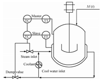
Ⅱ. THE CHYLLA-HAASE BENCHMARK A. The Polymerization ReactorThe industrial polymerization process described by Chylla and Haase[1, 2] consists of a stirred tank reactor with a cooling jacket and a coolant recirculation; as shown in Fig. 1. The reactor temperature is maintained at its setpoint by adjusting the coolant temperature,which is recirculated through the cooling jacket. There is a typical cascade control loop in practice and the purpose of this work is to design the outer loop controller. The slave controller for the jacket temperature has already been designed,which is a split-range proportional integral controller. The slave can act in two different modes: cooling mode (Cold water is inserted into the recirculation loop for controller outputs less than 50 %) and heating mode (Medium pressure steam is injected into the recirculating water stream when controller outputs greater than 50 %). Chylla and Haase give data for two different products A and B,whose recipe and process are slightly different. Here just product A is considered. The polymerization process is an exothermic reaction under specific recipe and process[6] which are given below.
|
Download:
|
| Fig. 1. The schematic diagrams of the polymerization reactor. | |
First,the given initial charges of solids (prepolymer,monomer) and water are fed into the reactor at the ambient temperature, $T_{\rm amb}$. The polymerization reaction has multi-phase consisting the heating phase from 0 s to 1 800 s,feeding phase from 1 800 s to 6 000 s,and the holding phase from 6 000 s to 9 600 s.
1) At the heating phase,the temperature of initial charges is raised to the reaction temperature setpoint $T^{\rm set}$ at 1 800 s. Generally,the desired trajectory of temperature increasing according to the given setpoint $T^{\rm set}$ is defined as
| \begin{align} T^{*}(t)= \left\{ \begin{array}{llll} T_{\rm amb}+(T^{\rm set}-T_{\rm amb})\displaystyle\sum_{i=3}^{5}a_{i}(\frac{t}{t^{\rm heat}})^i,&t\leq t^{\rm heat},\\ T^{\rm set},&t>t^{\rm heat}, \end{array} \right. \label{eq1} \end{align} | (1) |
2) At the feeding phase from 1 800 s to 6 000 s,pure monomer is fed into the reactor at $7.560\times 10^{-3} {\rm kg/s}$ until 6 000 s. Polymerization reaction begins and the large amount of heat is released. So the reactor temperature should be heated from ambient temperature to setpoint $T^{\rm set}$ according to the desired trajectory $T^*(t)$.
3) During the holding phase from 6 000 s to 9 600 s,the monomer feed ends abruptly,and exothermic reaction continues. The reactor temperature also should be held at its setpoint until the batch ends.
| \begin{align} \frac{{\rm d}m_{M}}{{\rm d}t}=\dot{m}_{M}^{\rm in}(t)+\frac{Q_{\rm rea}}{\delta H} ,\label{eq2} \end{align} | (2) |
| \begin{align} \frac{{\rm d}m_{P}}{{\rm d}t}=-\frac{Q_{\rm rea}}{\delta H}, \label{eq3} \end{align} | (3) |
| \begin{align} \begin{split} \frac{{\rm d}T}{{\rm d}t}=&\frac{1}{\displaystyle\sum_{i}m_{i}C_{p,i}}[\dot{m}_{M}^{\rm in}(t)C_{p,M}(T_{\rm amb}-T)-UA(T-T_j)-\\ &(UA)_{\rm loss}(T-T_{\rm amb})+Q_{\rm rea}],\quad i=M,P,W, \end{split}, \end{align} | (4) |
| \begin{align} &\frac{{\rm d}T_{j}^{\rm out}}{{\rm d}t}=\frac{1}{m_{c}C_{p,C}}\times\notag\\ &\quad[\dot{m}_{c}C_{p,C}(T_{j}^{\rm in}(t-\theta_{1})-T_{j}^{\rm out})+UA(T-T_{j})],\label{eq5} \end{align} | (5) |
| \begin{align} \frac{T_{j}^{\rm in}}{{\rm d}t}=\frac{{\rm d}T_{j}^{\rm out}(t-\theta_{2})}{{\rm d}t}+\frac{T_{j}^{\rm out}(t-\theta_{2})}{\tau_{p}}+\frac{K_{p}(c)}{\tau_{p}}. \label{eq6} \end{align} | (6) |
A physical model of the polymerization reactor has been derived by Chylla and Haase based on the first order kinetic relation[5]. The reactor model comprises material balance and energy balance equations. The material balance equations describes the conversion from monomer $M$ to polymer P in water W,as shown in (2) and (3). Here,$m_{M}(t)$ and $m_{P}(t)$ are monomer mass and polymer mass, respectively. The temperature dynamics are captured by the energy balance equations for the reactor and the cooling jacket. The energy balance in (4) gives a dynamic relationship of reactor temperature $T(t)$,and (5) and (6) describe the temperature of cooling jacket outlet $T_{j}^{\rm out}$ and recirculation loop inlet $T_{j}^{\rm in}$ of coolant $C$,respectively. Furthermore,variables and parameters of reactor model are listed in Table I[6].
|
|
TABLE Ⅰ VARIABLES AND PARAMETERS OF REACTOR MODEL |
The differential equation for the cooling jacket temperature contains delay time $\theta_{1}$,and the recirculation loop dynamics are modeled with delay time $\theta_{2}$. The gain $K_{p}(c)$ of recirculation loop is split-range accounting for the difference in heating and cooling mode,i.e.,
| \begin{align} K_{p}(c)= \left\{ \begin{array}{lllll} 0.8\times30^{-\frac{c}{50}}(T_{\rm inlet}-T_{j}^{\rm in}(t)),&c<50%,\\ 0,&c=50%,\\ 0.15\times30^{-\frac{c}{50}}(T_{\rm stream}-T_{j}^{\rm in}(t)),&c>50%,\\ \end{array} \right. \label{eq7} \end{align} | (7) |
1) When $c>50 %$,the slave controller acts in the heating mode, the coolant is heated by injecting steam to the recirculating water stream in order to increase the temperatures of jacket and reactor;
2) When $c < 50 %$,the slave controller acts in cooling mode,the ice water is inserted to cooling jacket in order to decrease the temperatures;
3) When $c=50 %$,the steam valve and the dumping valve are closed,the water of jacket is circulating by itself.
Table II lists the empirical relation for $R_{p}$ (the polymerization rate),$A$ (the jacket heat transfer area) and $U$ (the overall heat transfer coefficient) taken from [5]. The model parameter values of polymer A are given in Tables III and IV[6].
|
|
TABLE Ⅱ EMPIRICAL RELATIONS FOR POLYMERIZATION RATE $R_{p}$, JACKET HEAT TRANSFER AREA $A$, AND OVERALL HERT TRANSFER COEFFICIENT $U$ |
|
|
TABLE Ⅲ DATE FOR REACTOR PARAMETERS |
|
|
TABLE Ⅳ DATE FOR POLYMER A |
According to the description of recipe and process for polymerization product A[1, 2],the control tasks are developed:
1) Heating the reactor temperature $T(t)$ to a constant set point $T^{\rm set}$ in accordance with the reference trajectory $T^*(t)$ (1) before the monomer feed starts. The tracking error is not exceeding $\pm~0.6$ K.
2) Keeping the reactor temperature $T(t)$ within a maximum tolerance deviation of $\pm~0.6$ K during the monomer feeding period and the temperature holding period in which the monomer feed is finished.
It is described in the recipe that polymer A is produced in five subsequent batches and removed between the batches. However,this reaction is not a traditional batch process. Polymer viscosity increases continuously and significantly during a batch. Furthermore,the polymer will be surface fouling on the reactor wall because the reactor is only cleaned after the fifth batch. These lead the heat transfer coefficient to fall sharply during the following batch. The heat transfer coefficient is a key parameter,whose time-varying and batch-varying characters in the system model must be taken into account. In addition,some other given physical property data,such as impurity factor,are different from the first batch. So the traditional control method,such as PID and traditional ILC,is not suitable to solve the highly precise tracking problem for the shifty system model.
In brief,the reaction kinetics of Chylla-Hasse bechmark are complex and highly nonlinear. Generally,the control aporia consists of batch (and/or time)-varying process model and complex extra-disturbance. First,the batch (and/or time)-varying character of reaction dynamic system is shown in the following:
1) Impurity factor $i\in [0.8,1.2]$ in the polymerization rate $R_{p}$ is random at different batches,and it is usually constant during one batch. The impurity factor shows the purity of the monomer which will affect the terminal produce quality. It is a common problem in the practical process.
2) Fouling factor $1/h_{f}$ increases during a batch and from batch to batch due to an increasing polymer viscosity. So the overall heat transfer coefficient $U$ will fall correspondingly.
3) Delay times $\theta_{1}$ and $\theta_{2}$ of the cooling jacket may vary at $\pm~25 %$ compared to the nominal value at different batches.
Meanwhile,the extra-disturbances and uncertainties are complex and various. For example:
1) The monomer feed starts and ends abruptly at specified time points.
2) The ambient temperature $T_{\rm amb}$ is different during summer and winter,which influences reactor initial conditions. This is inconsistent with the basic hypothesis of traditional ILC,in which initial conditions should be the same at each different batch.
3) Measurement noise and other process noise also exist and affect the highly precise tracking control of reactor temperature.
Ⅲ. ADAPTIVE ITERATIVE LEARNING CONTROL BASED ON UNFALSIFIED STRATEGYThe Chylla-Hasse reaction is a kind of semi-batch process,which is different from the batch process in manufacturing industry because of its complex chemical reaction. The traditional iterative learning control (ILC) can not be directly applied to this reactor,and the reason has been analyzed as above mentioned. A superior control algorithm is desired to replace one or both of the PID controllers of Fig. 1 in order to solve the tight temperature control problem. Here an adaptive iterative learning control algorithm based on unfalsified strategy is proposed to replace the master controller,which can deal with chemical reaction process with complex reaction mechanism and batch (and/or time)-varying model. A close-loop P-type ILC is the fixed candidate controller structure,and the unfalsified strategy is adopted to adjust adaptively the learning rate of the P-type ILC controller.
It is known from the industrial recipe that the polymerization reactor is cleaned after every five sub-batches. At these five sub-batches,polymer A will be surface fouling on the reactor wall,then the heat transfer coefficient decreases along with the increasing of batch number. Then the initial condition and model dynamic of the each sub-batch is different (Here the impurity of monomer is considered as random noise). Therefore,the basic assumption of iterative learning control that initial condition of each batch should be same is not satisfied. The traditional ILC cannot be used directly in this problem.
In order to solve this problem,the adaptive iterative learning control based unfalsified strategy is proposed. Firstly,every five sub-batches of this polymerization reactor is considered as the different stage in one big process as shown in Fig. 2. Then the sub-batch number is defined as follows: \begin{align*} B_{k}^{i}=5(k-1)+i,k=1,2,\cdots,N,~i=1,2,3,4,5, \end{align*} where $k$ is the iterative number of big process and $i$ is the sequence number of the five batches in the big process. Then each sub-batch in the big process satisfies the basic assumption of ILC along with the iterative number of the big process. The initial condition of a sub-batch is the same in the view of the iterative axe,i.e.,$B_{k}^{i}(0)=B_{k+1}^{i}(0)$,because the reactor will be clean after the fifth batch. Moreover,there is another problem that should be considered: the dynamic character and initial condition of each sub-batch is different in a big process. So adaptive iterative learning control is given to regularize the learning gain of ILC in order to compensate the initial condition difference among different sub-batches. The structure of adaptive ILC based on unfalsified strategy is shown in Fig. 3. The control scheme is separated into two layers. Closed-loop P-type adaptive ILC is the master controller in the upper layer,whose learning gain is adjusted by the unfalsified scheduler. The underlying is the slave PI controller,which aims at tightly tracking the reference temperature trajectory calculated by the master controller. Cost function values are calculated based on the input-output data in order to select the most suitable learning gain in the unfalsified scheduler. Then this gain is sent to the P-type ILC for next batch control. This control structure can adjust controller parameter adaptively and dynamically.

|
Download:
|
| Fig. 2. Introduction of big process. | |

|
Download:
|
| Fig. 3. Structure of adaptive iterative learning control based unfalsified strategy. | |
The batch process is obviously a 2-D system[25] whose dynamics propagates along the time as well as batch direction. As we known,the traditional unfalsified control is applied only to the time domain. Here,unfalsified control theory is extended from time to the iteration domain. The basic definitions and theorems about unfalsified control in time domain are given in [26, 27]. A controller is said to be falsified by measurement information if this information is sufficient to deduce that performance specification $(r,y,u)\in T_{\rm spec},\forall r\in {\bf R}$ will be violated when the controller is in the feedback loop. Otherwise,the controller is said to be unfalsified. There is another important concept of fictitious reference signal $\widetilde{r}$. Suppose that $K$ is a candidate controller which has been in the control system,then some input-output data $(u,y)$ can be collected. The fictitious reference signal $\widetilde{r}(K)$ is defined to be any signal with the property that if the reference signal $\widetilde{r}(K)$ had been applied to the system,then the measured data $(u,y)$ would have been reproduced.
A candidate controller $K(\theta)$ is judged to be unfalsified at time $t$ by plant data $u(\tau),y(\tau),(\tau\in[0,t])$ if and only if
| \begin{align} \widetilde{J}(\theta,\tau)=-\rho(\tau)+\int_{0}^{\tau}T_{\rm spec}(\widetilde{r}(\theta,\zeta),y(\zeta),u(\zeta)){\rm d}\zeta\leq 0,\label{eq8} \end{align} | (8) |
Similar to these basic concepts in time domain,the iteration unfalsiled control concepts are proposed here.
Iteration unfalsification. A candidate ILC is said to be falsification in the iterative direction by measurement information from prior batches if this information is sufficient to deduce the performance specification $(r_{k},y_{k},u_{k})\in T_{{\rm spec},k}, \forall r_{k}\in {\bf R}$ will be violated when this controller is in the feedback loop. Otherwise,the parameter of ILC is said to be unfalsified.
Fictitious reference signal ${\pmb{\widetilde{r}_{k}}}$ at ${\pmb k}$-th iteration. Given measured data $(u_{k},y_{k})$,the fictitious reference signal $\widetilde{r}_{k}(K)$ for each candidate controller $K$ is any signal with the property that if the candidate controller $K$ had been in the control system during the whole batch,when the input-output data $(u_{k}(\tau),y_{k}(\tau)), \tau\in[0,t_{f}]$ was collected,and the signal $\widetilde{r}_{k}(K,\tau)$ had been applied to the system,then the measured data $(u_{k},y_{k})$ would have been reproduced.
A candidate ILC is unfalsified at the $k$-th iteration by plant data $u_{k}(\tau),y_{k}(\tau),(\tau\in[0,t_{f}])$,if and only if
| \begin{align} &\widetilde{J}_k(\tau)=\notag\\ &\quad-\rho_{k}(\tau)+\int_{0}^{t_{f}}T_{{\rm spec},k}(\widetilde{r}_{k}(K,\tau),u_{k}(\tau),y_{k}(\tau)){\rm d}\tau\leq 0,\label{eq9} \end{align} | (9) |
We have defined the five sub-batch as a big process according to the recipe of Chally-Hasse polymerization. But a same learning rate is not suitable in this big process because the model of each sub-batch is different. The learning rate should be adjusted with the system condition and tracking error of the current sub-batch. So adaptive iterative learning control is developed to solve this problem. The unfalsified control driven by plant data is a new effective adaptive control method,which has been extended to the iterative domain stated in Section III-A. So the adaptive iterative learning control based on unfalsified strategy is described as following.
The close-loop P-type iterative learning control algorithm is selected because it is simple and effective for the control problem of Chally-Hasse polymerization. The control law is
| \begin{align} \begin{split} u_{k}(t)&=u_{k-1}(t)+R_{k}e_{k}(t),\\ e_{k}(t)&=y_{k}(t)-y_{d}(t), \end{split} \label{eq10} \end{align} | (10) |
The adaptive ILC (10) is the master controller in this polymerization problem,where $u_{k}$ is the setpoint of the cooling jacket temperature,and the output signal $y_{k}$ is the reactor temperature. So (10) can be written as
| \begin{align} \begin{split} T_{j,k}^{\rm set}(t)&=T_{j,k-1}^{\rm set}(t)+R_{k}e_{k}(t),\\ e_{k}(t)&=T_{k}(t)-T^{*}(t). \end{split} \label{eq11} \end{align} | (11) |
| \begin{align} R=\{R_{1},R_{2},\cdots,R_{m}\}. \label{eq12} \end{align} | (12) |
Then the appropriate learning rate $R_{k}$ is determined on-line by the unfalsified strategy according to the tracking error and system dynamic.
Firstly,an improved cost function is given,
| \begin{align} T_{{\rm spec},k}(t)=(\widetilde{r}_{k}(t)-y_{k}(t))^2-\omega\cdot {\rm e}^{-(y_{d}(t)-y_{k}(t))^{2}},\omega>0,\label{eq13} \end{align} | (13) |
Here the fictitious reference signal $\widetilde{r}_{k}$ is given based on its definition,
| \begin{align} \widetilde{r}_{k}=y_{k}+\frac{1}{R_{k}}(u_{k}-u_{k-1}). \label{eq14} \end{align} | (14) |
So the unfalsified switch function $J_k$ is shown as
| \begin{align} \begin{split} \widetilde{J}_k&=\int_{0}^{t_{f}}T_{\rm spec}(\tau){\rm d}\tau=\\ &\int_{0}^{t_{f}}((\widetilde{r}_{k}(\tau)-y_{k}(\tau))^2-\omega\cdot {\rm e}^{-(y_{d}(\tau)-y_{k}(\tau))^{2}}){\rm d}\tau. \end{split} \label{eq15} \end{align} | (15) |
| \begin{align} \widetilde{J}_k=\int_{0}^{t_{f}}((\widetilde{r}_{k}(\tau)-y_{k}(\tau))^2-\omega\cdot {\rm e}^{-(y_{d}(\tau)-y_{k}(\tau))^{2}}){\rm d}\tau\leq 0. \label{eq16} \end{align} | (16) |
The tracking error is very large at the beginning of the iterative process in general,so item ${\rm e}^{-(y_{d}(\tau)-y_{k}(\tau))^{2}}$ is very small. The unfalsified condition (16) is so strict that a few of the candidate learning gains can satisfy this condition. At that time, the learning gains that satisfy unfalsified condition are those relatively larger,even the maximum in the candidate set. According to the principle of minimum-selected,the minimum is selected as the most suitable gain in the next iteration. Then the tracking error of the next iteration will decrease rapidly,when the selected controller is in the feedback loop. Then item ${\rm e}^{-(y_{d}(\tau)-y_{k}(\tau))^{2}}$ becomes lager due to the decreasing of trace error. The unfalsified condition is relaxed, and there are more gains in the candidate learning gain set satisfying this condition. Generally,the selected controller gain is gradually reduced with the increasing of iteration number. So the iterative learning controller is self-adjusting to adapt different error levels.
C. The Initial Control in Iterative Learning ControlThe Chylla-Haase reactor is a kind of typical practical equipment, and a very tight temperature control is necessary in order to achieve the desired product quality. The controller should be able to maintain the reactor temperature $T$ around the desired set-point in an interval of $\pm 0.6$ K under all operation conditions and disturbances. The initial control will influence the product quality in the first iteration as well as the convergence speed of tracking error. Actually,the initial control is an important problem in iterative learning control,but it is always omitted. Most research about ILC focus on the design of control law and it convergence condition. How to get the appropriate initial temperature of the jacket (i.e.,the initial controller output) is necessary for the convergence of the adaptive ILC algorithm and industrial demand. Here the reaction mechanism as prior knowledge is usually used to design initial controller according system model (2) $\sim$ (6)[5].
The energy balance (4) gives a dynamics relationship between system input (cooling jacket temperature $T_j$) and output (reactor temperature $T$),which can be abbreviated to
| \begin{align} \dot{T}=\alpha(\dot{m}_{M}^{\rm in}(t),m_{M},m_{P},T,T_{j}). \label{eq17} \end{align} | (17) |
| \begin{align} T_{j}^{*}=\alpha^{-1}(\dot{m}_{M}^{\rm in}(t),m_{M}^{*},m_{P}^{*},T^{*}(t),\dot{T}^{*}(t)) \label{eq18} \end{align} | (18) |
| \begin{align} \begin{split} \dot{m}_{M}^{*}&=\beta_{M}(\dot{m}_{M}^{in}(t),m_{M}^{*},M_{P}^{*},T^{*}),m_{M}^{*}(0)=m_{M,0},\\ \dot{m}_{P}^{*}&=\beta_{P}(\dot{m}_{M}^{in}(t),m_{M}^{*},M_{P}^{*},T^{*}),m_{P}^{*}(0)=m_{P,0}. \label{eq19} \end{split} \end{align} | (19) |
So the initial temperature trajectory of cooling jacket $T_{j}^{*}$ (initial input) is given in (18) and (19). It is completely dependent on the reactor mechanism,which guarantees produce quality in the initial iteration.
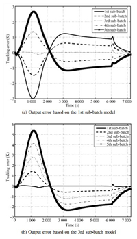
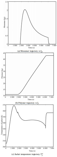
By recalling that we have defined the sequential five sub-batches as a big process in the last section,and that the iterative learning control is used to decrease output error,it is not necessary to calculate $T_{j}^{*}$ of each batch. Then there is an important question to be answered. Which sub-batch mechanism model is the most appropriate. As we know that they are very different due to the polymer viscosity increasing and fouling. If the mechanism model of first sub-batch is adopted,the initial error will increase with the sub-batch number in the first big process. The error of the 5th batch is too large to be tolerable as shown in Fig. 4 (a). The heat transfer coefficient decreases with the batch number,so we choose $T_{j}^{*}$ of the 3rd batch as the initial law of controller in the first big process. The relative results about third sub-batch are given in Fig. 4 (b). It is shown that the output error in each sub-batch is allowable and compromised. The calculated trajectories of $m_{M}^{*}$, $m_{P}^{*}$ and $T_{j}^{*}$ according to the third sub-batch mechanism are shown in Fig. 5.
|
Download:
|
| Fig. 4. The performance comparison in one big process under different initial jacket temperature. | |
|
Download:
|
| Fig. 5. The initial condition of Chylla-Haase process. | |
Actually,the initial temperature trajectory of the cooling jacket is not a necessary convergence condition for the proposed adaptive ILC control. But if the initial input of first iteration is arranged as (18),the tracking error will be convergent to the desired level as fast as possible. The initial input can be selected according to the practical experiences when there are not exact mechanism model information of the process.
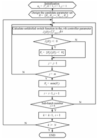
D. Summary of the Control AlgorithmThe implementation procedure for the proposed adaptive iterative learning based on unfalsified strategy is summarized in the following. The algorithm flow chart is shown in Fig. 6.
|
Download:
|
| Fig. 6. Flow chart of adaptive ILC control. | |
Step 1. The initial temperature of jacket $T_{j}^{*}$ (18) is calculated according to the reaction mechanism,which is arranged as the initial output of the master controller for the first iteration,
| \begin{align} u_{0}=T_{j}^{*}.\label{eq20} \end{align} | (20) |
Step 2. The candidate parameter set of adaptive P-type ILC controller is given according to the convergence condition, which will be discussed in the next subsection.
| \begin{align} R=\{R_{1},R_{2},\cdots,R_{m-1},R_{m}\}. \label{eq21} \end{align} | (21) |
Step 3. The unfalsified switch function $\widetilde{J}_{k}$ (15) is calculated respectively for every element $R_{i},i=1, \cdots,m$ in the candidate parameter set $R$ when each sub-batch ends.
Step 4. The parameters set whose elements all satisfy the unfalsified condition is defined as $R_{s}$ \begin{align*} R_{s}=\{R_{i}\mid \widetilde{J}_{k}(R_{i}) < 0\}. \end{align*}
Then the minimum in the parameters set $R_{s}$ is selected as the most suitable learning rate for next iteration,that is \begin{align*} R_{k+1}={\rm min}(R_{s}). \end{align*}
Step 5. The new learning rate is inserted to next iteration P-type ILC in each sub-batch,and the above steps from Step 3 are repeated.
E. Convergence AnalysisThe proposed method is actually a closed-loop P-type ILC,and the unfalsified strategy is only for the self-tuning of controller gain. So the unfalsified strategy will not influence the convergence of the proposed control algorithm. Generally,the controller gain $R_{i},i=1,\cdots,m$ in the candidate parameter set should satisfy the convergence condition of the tradition ILC. But this constraint can be relaxed here because of the unfalsified strategy.
We have defined the candidate parameter set in prior section,and the maximum and minimum gains are found, \begin{align*} \begin{split} &R=\{R_{1},R_{2},\cdots,R_{m-1},R_{m}\},\\ &R_{\max}=\max\{R_{i}\},i=1,\cdots,m ,\\ &R_{\min}=\min\{R_{i}\}. \end{split} \end{align*}
To describe the convergence condition of the control algorithm,a general model of the Chylla-Haase reaction is considered. In the above,we defined the five sub-batch in the Chylla-Haase process as the five different stages in the big process,so we transform batch-varying of parameters from sub-batch to time-varying in the big process. So we select a nonlinear time-varying mathematical model to analyze the convergence.
| \begin{align} \begin{split} \dot{x}_{k}(t)&=f(t,x_{k})+B(t)u_{k}(t),\\ y_{k}(t)&=g(t,x_{k})+D(t)u_{k}(t), \end{split} \label{eq22} \end{align} | (22) |
Here we consider the constraint of the candidate controller gain $R_{k}$ to ensure the uniform convergence of the tracking error along with the iteration index.
For given a system (22) and desired output trajectory $y_d(t)$, the adaptive iterative learning controller is (10),(20) and (21). If the following conditions are satisfied,
1) The maximum gain $R_{\rm max}$ should satisfy that the close-loop system is stable and $L_{2}$-norm of tracing error of the second iteration is less than that of the first iteration, that is where $||e(t)||^{2}=\int_{0}^{T_f}e(t)e^{\rm T}(t){\rm d}t=\int_{0}^{T_f}(y_d(t)-y(t))(y_d(t)-y(t))^{\rm T}{\rm d}t$,and subscripts 1 and 2 mean the first and the second iterations, respectively.
| \begin{align} ||e_{2}||^{2} < ||e_{1}||^{2},\label{eq23} \end{align} | (23) |
2) The minimum $R_{\min}$ should satisfy the convergence condition of traditional close-loop P-type ILC,which is discussed in [28], i.e.,
| \begin{align} \begin{split} ||(I+D(t)R_{\min})^{-1}|| < 1, \end{split} \label{eq24} \end{align} | (24) |
Analysis.
Here the iterative learning controller is a proportional controller. The tracking error is commonly vary large at the first iteration,so the maximum gain $R_{\max}$ must be selected. Then the tracking error is decreasing at the following iteration due to iterative control,i.e.,the condition $||e_{2}||^{2} < ||e_{1}||^{2}$ is satisfied. It is obviously that the unfalsified condition (16) is loose,and the parameter set $R_s$ whose elements all satisfy the unfalsified condition becomes bigger. Then the learning gain of next iteration must be smaller than that of first iteration based on the rule of minimum-selection in set $R_s$,
| \begin{align} R_{2}\leq R_{\max}.\label{eq25} \end{align} | (25) |
If the convergence condition (1) is satisfied,the maximum controller gain $R_{\max}$ makes the close-loop system stable and the tracking error decreases during the two adjacent batch. So any controller gain $R\leq R_{\max}$ also can assure the close-loop system stable. The parameter set $R_s$ which satisfies the unfalsified condition will become bigger with the decreasing of tracking error,and the learning rate will continue to get smaller. Then we know that the controller gain in the following iteration has the following relationship
| \begin{align} R_{\min}\leq R_{N}\leq R_{N-1}\leq \cdots\leq R_2 \leq R_1=R_{\max},\label{eq26} \end{align} | (26) |
| \begin{align} \lim_{k\rightarrow\infty}(y_{d}(t)-y_{k}(t))=0. \label{eq27} \end{align} | (27) |
According to (14),we can obtain
| \begin{align} \begin{split} &\lim_{k\rightarrow\infty}(\widetilde{r}_{k}(t)-y_{k}(t))=\\ &\quad \lim_{k\rightarrow\infty}\frac{1}{R_{k}}(u_{k}-u_{k-1}). \end{split} \label{eq28} \end{align} | (28) |
When the tracking error is convergent,the output of the controller is convergent
| \begin{align} \begin{split} \lim_{k\rightarrow\infty}(u_{k}-u_{k-1})=0,\\ \lim_{k\rightarrow\infty}(\widetilde{r}_{k}(t)-y_{k}(t))=0. \end{split} \label{eq29} \end{align} | (29) |
According to (27) and (29),we have
| \begin{align} \begin{split} &\lim_{k\rightarrow\infty}T_{\rm spec}(\widetilde{r}_{k}(t),y_{k}(t),u_{k}(t))=\\ &\quad \lim_{k\rightarrow\infty}((\widetilde{r}_{k}(t)-y_{k}(t))^2-w{\rm e}^{-(y_{d}(t)-y_{k}(t))^2})=\\ &\quad\lim_{k\rightarrow\infty}(0-w\times1)=-w < 0, \end{split} \label{eq30} \end{align} | (30) |
| \begin{align} \lim_{k\rightarrow\infty}\widetilde{J}_k=\lim_{k\rightarrow\infty}\int_{t_{0}}^{t_{f}}T_{\rm spec}{\rm d}t=-w < 0.\label{eq31} \end{align} | (31) |
| \begin{align} \lim_{k\rightarrow\infty}R_{k}=R_{\min}. \label{eq32} \end{align} | (32) |
At the same time,if $R_{\min}$ satisfies the iterative convergence condition of traditional P-type ILC,i.e.,(24),the adaptive ILC algorithm based on unfalsifed strategy is uniformly convergent.
In practical application,$R_{\min}$ is selected according to (24) which is the convergence condition of P-ILC. Here the parameter $D(t)$ is a static gain which can generally be obtained by experiment even if the control plant is unknown; and $R_{\max}$ is selected to satisfy (23) according to engineer experience as the same as the traditional proportion controller. The main aim of $R_{\max}$ is to assure the tracking error decreasing rapidly in the first couple of iterations.
Ⅳ. SIMULATION RESULTS AND DISCUSSIONSThe adaptive iterative learning control based unfalsified strategy is applied to a semi-batch Chylla-Haase process. Simulation parameters are listed in the following:
1) Original candidate parameter set:
R=[1, 4, 5, 8, 9, 12, 10, 16, 18, 2, 3, 20].
2) Slave PI controller parameters: $K_{P}=20,K_{I}=1$.
3) Pre-tuning integer: $\omega$ = 0.01.
4) Sampling time: $t_{s} = 4$ s.
According to the mechanism model,the uncertainty of the process includes two aspects: impurity of monomer which changes randomly between 0.8 and 1.2,and decreasing of coefficient after each sub-batch,which is a time-varying parameter in the big process. These parameters are described in Table III.
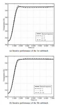
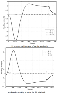
Control performances based on the proposed adaptive ILC are showed in Figs. 7 and 8,in which the reactor temperature and tracking error trajectories of the 1st and 5th sub-batch in one big process are given respectively. It is shown that the control performance is very bad and the tracking errors is far more than the tolerance of 0.6 K at the first iterative big process. This is because the initial output of the controller is calculated by the mechanism model of the 3rd sub-batch,which is clearly different from the 1st and 5th sub-batch due to surface fouling. Although the parameters of the model have changed between the 1st sub-batch and 5th batch,the tracking performance is continuously improved due to the proposed iterative controller. The tracking errors decrease fast and the accurate tracking performance has been achieved quickly.
|
Download:
|
| Fig. 7. Control performance of the proposed adaptive ILC. | |
|
Download:
|
| Fig. 8. Tracking error of the proposed adaptive ILC. | |
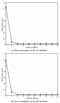
The convergence trajectory of mean square error along the iterative axis is shown in Fig. 9. The convergent speed of error under the proposed adaptive ILC controller is very fast. At the same time,it can be seen that every close-loop system during the iterative control is stable,and mean square error is convergent to zero at the third iteration.
|
Download:
|
| Fig. 9. Error convergence of the proposed adaptive ILC. | |
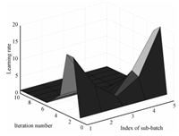
The change of the learning gain in each sub-batch is showed in Fig. 10. The initial condition of $i$-th sub-batch $B_k^i$ along the iterative number $k$ is the same,so iterative learning control for each sub-batch can be applied. The learning gain for each sub-batch is determined adaptively according to the proposed adaptive ILC algorithm. These sub-batch learning rates are different because the model of each sub-batch in one big process is different. Furthermore,the initial errors of the 1st and the 5th sub-batch are large because the initial controller $u_0$ is calculated based on the 3rd sub-batch mechanism model,so the learning gain in the first iterative process is large. Then the learning gain decreases and is convergent to the minimum $R_{\min}$ with the decreasing of tracking error.
|
Download:
|
| Fig. 10. The change of the learning rate in each batch. | |
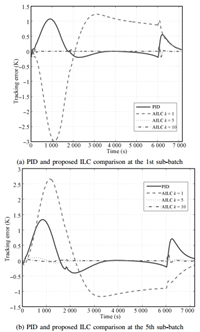
The control performance comparison between the traditional PID controller and the proposed adaptive ILC controller is shown in Fig. 11. Also the results of the 1st and the 5th sub-batch are given. The tracking error under PID controller remains unchanged along the iteration axes because it does not have the iteratively improved ability,while the tracking errors under three different iteration ($k$ = 1,3,5) of the adaptive ILC are shown in Fig. 11. Although the performance of PID is better than that of the AILC in the first iteration,the error under PID controller does not satisfy the control requirement (tolerance of $\pm 0.6$ K),and the error does not decrease with iteration increasing. However,under the control of adaptive ILC,the errors decrease rapidly to the tolerance zone in spite of the initial tracking error is larger than that of the PID control. As the traditional PID control does not decrease the tracking error along the iteration axi,the final control performance is far worse than that of adaptive ILC.
|
Download:
|
| Fig. 11. Results comparison between PID and adaptive ILC. | |
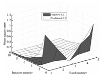
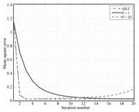
Furthermore,the control performance comparison between the traditional ILC and the proposed adaptive ILC is given in Figs. 12 and 13. It is shown that the convergent speed of the adaptive ILC is obviously faster than that of the traditional ILC, and the control performance is also better. The control results of two different controller gains ($R=1$ and $R=20$) are given during the test of traditional ILC. These two gains are corresponding to the maximum and minimum gains ($R_{\min}$ and $R_{\max}$) in adaptive ILC,respectively. In the case of the controller gain $R=1=R_{\min}$,the mean square error continues to fall and converges to zero at the 20th iteration,obviously the convergence speed is very slow. In another case of the controller gain $R=20=R_{\max}$,the mean square error converges fast at the beginning,but it is divergent finally when the iteration process increases. This is because a bigger gain usually does not satisfy the convergence conditional (24). The adaptive ILC shows good performance compared with the traditional ILC: fast convergence speed,uniform convergence and relaxed controller gain condition.
|
Download:
|
| Fig. 12. Convergence speed comparison of adaptive ILC and traditional ILC. | |
|
Download:
|
| Fig. 13. Mean square error trajectory of adaptive ILC and traditional ILC. | |
An adaptive iterative learning control based on unfalsified strategy is proposed to solve the accurate tracking problem in the Chally-Haase polymerization process. The core of the proposed algorithm is adaptively adjusting the learning gain of P-type ILC according to the unfalsified strategy. The unfalsified control strategy is extended from the time domain to the iteration domain, and the basic definition and mathematics description of unfalsified control in the iteration domain are given. Furthermore,two important problems in iterative learning control,i.e.,the initial control law and convergence analysis,are discussed in detail. The initial input of the first iteration is arranged according to the 3rd sub-batch mechanism model,which can assure good produce quality in the first iteration. And it will improve the convergence speed of tracking error. The convergence condition of the proposed adaptive ILC is given,which is obviously relaxed compared with the traditional ILC.
This method is completely driven by process data. The process data of past batches (history data) are used to calculate the fictitious reference signal in order to evaluate these gains in the candidate gain set which is the most suitable learning rate for the next batch. In addition,the process data of the current batch (real-time data) are also used to build the control law of the adaptive ILC, which is proportional to the current measurement error. The control performance of the proposed algorithm is compared with the traditional ILC algorithm and common PID controller. The simulation results fully demonstrate that the temperature of polymerization reactor can converge to the desired temperature trajectory rapidly and tightly remain in the tolerance zone. The good performance of accurate dynamic tracking and stable convergence are verified. This algorithm is totally driven by process data without any information and assumption about the process model,so it is convenient to be applied to other similar complex industrial process whose model is with uncertainty and time (or batch)-varying parameters.
| [1] | Chylla R W, Haase D R. Temperature control of semi-batch polymerizationreactors. Computers & Chemical Engineering, 1993, 17(3):257-264 |
| [2] | Chylla R W, Haase D R. Temperature control of semi-batch polymerizationreactors (corrigenda). Computers & Chemical Engineering, 1993,17(3): 1213 |
| [3] | Finkler T F, Kawohl M, Piechottka U, Engell S. Realization of onlineoptimizing control in an industrial polymerization reactor. In: Proceedingsof the 8th IFAC International Symposium on Advanced Control ofChemical Processes. Furama Riverfront, Singapore: IFAC, 2012, 8(1):11-18 |
| [4] | Clarke-Pringle T, Macgregor J F. Nonlinear adaptive temperature controlof multi-product, semi-batch polymerization reactors. Computers & Chemical Engineering, 1997, 21(12): 1395-1409 |
| [5] | Graichen K, Hagenmeyer V, Zeitz M. Feedforward control with onlineparameter estimation applied to the Chylla-Haase reactor benchmark.Journal of Process Control, 2006, 16(7): 733-745 |
| [6] | Vasanthi D, Pranavamoorthy B, Pappa N. Design of a self-tuning regulatorfor temperature control of a polymerization reactor. ISA Transactions,2012, 51(1): 22-29 |
| [7] | Rani K Y. Sensitivity compensating nonlinear control: exact model basedapproach. Journal of Process Control, 2012, 22(3): 564-582 |
| [8] | Finkler T F, Lucia S, Dogru M B, Engell S. Simple control schemefor batch time minimization of exothermic semibatch polymerizations.Industrial & Engineering Chemistry Research, 2013, 52(17): 5906-5920 |
| [9] | Ahn H S, Chen Y Q, Moore K L. Iterative learning control: briefsurvey and categorization. IEEE Transactions on Systems, Man, andCybernetics, Part C: Applications and Reviews, 2007, 37(6): 1099-1121 |
| [10] | Wang Y Q, Doyle F J III, Gao F R. Survey on iterative learning control,repetitive control, and run-to-run control. Journal of Process Control,2009, 19(10): 1589-1600 |
| [11] | Lee K S, Lee J H. Iterative learning control applied to batch processes:an overview. Control Engineering Practice, 2007, 15(10): 1306-1318 |
| [12] | Chi R H, Hou Z S, Xu J X. Adaptive ilc for a class of discrete-timesystems with iteration-varying trajectory and random initial condition.Automatica, 2008, 44(8): 2207-2213 |
| [13] | Zhang Yu-Dong, Fang Yong-Chun. Learning control for systems withsaturated output. Acta Automatica Sinica, 2011, 37(1): 92-98 (inChinese) |
| [14] | Choi J Y, Lee J S. Adaptive iterative learning control of uncertain roboticsystems. IEE Proceedings Control Theory & Applications, 2000, 147(2):217-223 |
| [15] | Sun Ming-Xuan, Li Zhi-Le, Zhu Sheng. Varying-order sampled-dataiterative learning control for MIMO nonlinear systems. Acta AutomaticaSinica, 2013, 39(7): 1027-1036 (in Chinese) |
| [16] | Norrlof M. An adaptive iterative learning control algorithm with experimentson an industrial robot. IEEE Transactions on Robotics andAutomation, 2002, 18(2): 245-251 |
| [17] | Bu Xu-Hui, Yu Fa-Shan, Hou Zhong-Sheng, Wang Fu-Zhong. Iterativelearning control for a class of linear discrete-time switched systems.Acta Automatica Sinica, 2013, 39(9): 1564-1569 (in Chinese) |
| [18] | Chien C J, Yao C Y. Iterative learning of model reference adaptive controllerfor uncertain nonlinear systems with only output measurement.Automatica, 2004, 40(5): 855-864 |
| [19] | French M, Rogers E. Non-linear iterative learning by an adaptivelyapunov technique. International Journal of Control, 2000, 73(10):840-850 |
| [20] | Xu J X, Tan Y. A composite energy function-based learning control approachfor nonlinear systems with time-varying parametric uncertainties.IEEE Transactions on Automatic Control, 2002, 47(11): 1940-1945 |
| [21] | Kuc T Y, Han W G. An adaptive PID learning control of robotmanipulators. Automatica, 2000, 36(5): 717-725 |
| [22] | Afshar P, Wang H. ILC-based adaptive minimum entropy control forgeneral stochastic systems using neural networks. In: Proceedings ofthe 46th IEEE Conference on Decision and Control. New Orleans, USA:IEEE, 2007.252-257 |
| [23] | Shi Jia, Jiang Qing-Yin, Cao Zhi-Kai, Zhou Hua, Gao Fu-Rong. Twodimensionalmodel predictive iterative learning control scheme based ona two-dimensional performance model. Acta Automatica Sinica, 2013,39(5): 565-573 (in Chinese) |
| [24] | Stefanovic M, Safonov M G. Safe adaptive switching control: stabilityand convergence. IEEE Transactions on Automatic Control, 2008, 53(9):2012-2021 |
| [25] | Fang Y, Chow T W S. 2-D analysis for iterative learning controller fordiscrete-time systems with variable initial conditions. IEEE Transactionson Circuits and Systems, I: Fundamental Theory and Applications, 2003,50(5): 722-727 |
| [26] | Safonov M G, Tsao T C. The unfalsified control concept and learning.IEEE Transactions on Automatic Control, 1997, 42(6): 843-847 |
| [27] | Wang R R, Safonov M G.The Comparison of Unfalsified Control and Iterative Feedback Tuning, Technical Report, Department of ElectricalEngineering, University of Southern Calif. USA, 2002 |
| [28] | Rogers E, Galkowski K, Owens D H. Control Systems Theory andApplications for Linear Repetitive Processes. Berlin: Springer-Verlag,2007.41-83 |
 2014, Vol.1


