I. INTRODUCTION

Iterativelearning control (ILC) is an intelligent control method of humanoid thinking,which is especially suitable for dynamic processes or systems with the repetitive operation characteristics over a finite time interval^[1]. The main feature of ILC is that it can improve the tracking accuracy by adjusting the system input signal from one repetition cycle to another based on the error observation in each cycle. In addition,ILC has an advantage that it can design the controller with the imprecise dynamic characteristics of the controlled object or without any model. Currently,ILC is playing an important role in practice,such as robotic manipulator^[2],intelligent transportation systems^{[3, 4]},biomedicine^[5],etc.

Meanwhile,ILC is a branch of an intelligent control with strict mathematical description,and one of its basic research issues is to design the learning algorithm and analyze its convergence. Nowadays,the research results of iterative learning control on ordinary differential systems and difference systems are very fruitful. The research objects of ILC include linear systems,nonlinear systems,time-delay systems,fractional order systems,discrete systems,singular systems,etc. In terms of iterative learning control algorithm,there are P,D,PD,PID algorithms and their corresponding open-loop algorithms,close-loop algorithms,high-order algorithms,etc. (see ^[1],^{[6, 7, 8, 9, 10, 11, 12, 13, 14]}). However,there are not many research results of ILC for distributed parameter systems described by the partial differential equations. In ^[15],a first order hyperbolic distributed parameter system was discussed,using a set of ordinary differential equations to approximate the studied partial differential equations and designing the P-type iterative learning algorithm for the ordinary differential system such that the close-loop system is stable and satisfies the appropriate performance index. A class of second order hyperbolic elastic system was studied in ^[16],by using the differential difference iterative learning algorithm. In ^[17],P-type and D-type iterative learning algorithms based on semigroup theory were designed for a class of parabolic distributed parameter systems. Tension control system was studied in ^[18] by using the PD-type learning algorithm. In ^[19],by employing the P-type learning control algorithm,a class of single-input single-output coupling (consisting of the hyperbolic and parabolic equations) nonlinear distributed parameter systems were studied and convergence conditions,speed and robustness of the iterative learning algorithm were discussed. Recently,without any simplification or discretization of the 3D dynamics in the time,space as well as iteration domain,the ILC for a class of inhomogeneous heat equations was proposed in ^[20]. In addition,in ^[15] iterative learning for the distributed parameter systems were specifically studied while the learning algorithm was open-loop P-type. However,to the best of our knowledge,the related research achievement on the distributed parameter systems with close-loop learning algorithm has not yet appeared.

The close-loop iterative learning algorithm was first proposed in ^[21],which was used by many scholars for the iterative learning control problem of ordinary differential or difference systems later^[11]. The main characteristic of the close-loop iterative learning algorithm is to control signals associated with the current error information,which is different from open-loop iterative learning algorithm.

In this paper,a close-loop P-type iterative learning algorithm is proposed for linear parabolic distributed parameter systems,which covers many important industrial processes such as heat exchanger,industrial chemical reactor and biochemical reactor. And a complete proof of the convergence of iterative error is given. The main contributions in the paper are: 1) it is the first to use the close-loop learning algorithm to research distributed parameter system; 2) tracking error convergence analysis is given in detail,which involves three different domains: time,space,and iteration; 3) Employing difference method for partial differential equations,it gives the simulation examples.

II. PROBLEM STATEMENT AND NEW ALGORITHM

Consider an uncertain linear parabolic distributed parameter system with repetitive operation characteristics as follows^[8]:

$\left\{ \begin{array}{l} \frac{{\partial {q_k}(x,t)}}{{\partial t}} = D\Delta {q_k}(x,t) + A(t){q_k}(x,t) + \\ B(t){u_k}(x,t),\\ {y_k}(x,t) = C(t){q_k}(x,t) + G(t){u_k}(x,t), \end{array} \right.$

(1)

where subscript $k$ denotes the iterative number of the process; $x$ and $t$ respectively denote space and time variables,$(x,t)\in \Omega \times [0,T]$; $\Omega$ is a bounded open subset with smooth boundary $\partial\Omega$; $~{\pmb q}_k(\cdot,\cdot)\in \mathbf{R}^n$,${\pmb u}_k(\cdot,\cdot)\in \mathbf{R}^u$,${\pmb y}_k(\cdot,\cdot)\in \mathbf{R}^y$ are the state vector,input vector and output vector of the system,respectively; $A(t),B(t),C(t),G(t)$ are the bounded time-varying uncertain matrices with appropriate dimensions,$D$ is a bounded positive constant diagonal matrix,i.e.,$D=\text{diag}\{d_1,d_2,\cdots,d_n\}$,$0

The corresponding initial and boundary conditions of system (1) are

$\alpha {q_k}(x,t) + \beta \frac{{\partial {q_k}(x,t)}}{{\partial \nu }} = 0,(x,t) \in \partial \Omega \times [0,T],$

(2)

${q_k}(x,0) = {q_{k0}}(x),x \in \Omega ,$

(3)

where $\frac{\partial}{\partial {\pmb \nu}}$ is the unit outward normal derivative on $\partial\Omega$,${\alpha}$ and ${ \beta}$ are known constant diagonal matrices,satisfying

$$\begin{align*} &{\alpha}=\text{diag}\{\alpha_1 ,\alpha_2,\cdots,\alpha_n\},\alpha_i\geq 0,i=1,2,\cdots,n,\\ &{\beta}=\text{diag}\{\beta_1,\beta_2,\cdots,\beta_n\},\beta_i >0,i=1,2,\cdots,n. \end{align*}$$

For the controlled object described by system (1),let the desired output be ${\pmb y}_d(x,t)$. Now,the aim is to seek a corresponding desired input ${\pmb u}_d(x,t)$, such that the actual output of system (1)

$$ \begin{align*} {\pmb y}^{*}(x,t)=C(t){\pmb q}_d(x,t)+G(t){\pmb u}_d(x,t) \end{align*}$$

will approximate to the desired output ${\pmb y}_d(x,t)$. It is not easy to get the desired control for the system is uncertain. We will gradually gain the control sequence ${{\pmb u}_k(x,t)}$ by using the learning control method,such that

$$ \lim_{k \to \infty}{\pmb u}_k(x,t)={\pmb u}_d(x,t). $$

The close-loop P-type iterative learning control algorithm looking for the control input sequence ${{\pmb u}_k(x,t)}$ is

$\begin{align} {\pmb u}_{k+1}(x,t)={\pmb u}_k(x,t)+\Gamma(t){\pmb e}_{k+1}(x,t), \end{align}$

(4)

where the tracking error ${\pmb e}_{k+1}(x,t)={\pmb y}_d(x,t)-{\pmb y}_{k+1}(x,t)$,and $\Gamma(t)$ is the gain matrix in the learning process.

Assume that in the learning process,the system states start from the same initial value,i.e.,

$\begin{align} {\pmb q}_k(x,0)={\pmb q}_0(x),x \in \Omega ,k=1,2,\cdots, \end{align}$

(5)

or more generally,

${q_k}(x,0) = {\varphi _k}(x),x \in \Omega ,k = 1,2,\cdots ,$

(6)

$\left\| {{\varphi _{k + 1}}(x) - {\varphi _k}(x)} \right\|_{{L^2}}^2 \le l{r^k},r \in [0,1),l > 0.$

(7)

In this paper,the following notations are used.

For the $n$ dimensional vector $W=(w_1,w_2,\cdots,w_n)^{\rm T}$,its norm is defined as $\|W\|=\sqrt{\sum_{i=1}^{n}w_i^2}$. The spectrum norm of the $n \times n$-order square matrix $A$ is $\|A\|=\sqrt{\lambda_{\max}(A^{\rm T}A)}$,where $\lambda_{\max}(\cdot)$ represents the maximum eigenvalue.

For $1\leq p\leq\infty$,${L}^p(\Omega)$ represents all measurable functions defined on the domain $\Omega$ and satisfying the conditions

$$\begin{array}{l} {\left\| \upsilon \right\|_{{L^p}}} = {\{ \int\limits_{_\Omega } {|\upsilon (x){|^p}{\rm{d}}x} \} ^{\frac{1}{p}}} < \infty ,1 \le p < \infty ,\\ {\left\| \upsilon \right\|_{{L^\infty }}} = {\rm{ess}}\mathop {\sup }\limits_{x \in \Omega } |\upsilon (x)| < \infty ,p = \infty . \end{array}$$

For every $i$,if $\upsilon_i(x)\in {L}^p(\Omega)$,then ${L}^p$ norm and ${L}^\infty$ norm of the vector function are ${\pmb \upsilon}(x)=\{\upsilon_1(x),\upsilon_2(x),\cdots,\upsilon_n(x)\}^{\rm T}$

$$\begin{array}{l} {\left\| \upsilon \right\|_{{L^p}}} = {\{ \int\limits_{_\Omega } {{{\left| {\upsilon (x)} \right|}^p}{\rm{d}}x} \} ^{\frac{1}{p}}} < \infty ,1 \le p < \infty ,\\ {\left\| \upsilon \right\|_{{L^\infty }}} = {\rm{ess}}\mathop {\sup }\limits_{x \in \Omega } |{\upsilon ^{\rm{T}}}(x)\upsilon (x)| < \infty ,p = \infty . \end{array}$$

For the positive integer $m\geq 1$ and $1\leq p\leq \infty$,${W}^{m,p}(\Omega)$ denotes the Sobolev space constituted by the functions $m$ times differential and $p$ times integral on $\Omega$^[22]. Specially,for $ \upsilon(x)\in W^{1,p}$,define

$$\begin{align*} \|\upsilon\|_{{W}^{1,p}}=\|\upsilon\|_{{L}^p}+\|\nabla \upsilon\|_{{L}^p}, \end{align*}$$

where $\nabla$ is the gradient operator.

III. ALGORITHM CONVERGENCE ANALYSIS

Before giving the main results,two lemmas are given as follows^[7]:

Lemma 1. If the constant sequence $\{b_k\}_{k\geq 0}$ converges to zero,and the sequence $\{Z_k(t)\}_{k\geq 0}\subset {C}[0,T]$ (continuous function space defined on $[0,T]$) satisfies

${Z_{k + 1}}(t) = \beta {Z_k}(t) + M({b_k} + \int_t^0 {{Z_k}(s){\rm{d}}s} ),$

(8)

then $\{Z_k(t)\}_{k \geq 0}$ uniformly converges to zero,when $k\rightarrow\infty$,where $M>0$,$0 \leq\beta<1 $ are constant.

Lemma 2. If $f(t)$ and $g(t)$ are two continuous nonnegative functions on $[0,T]$,and there exist nonnegative constants $q$ and $M$ satisfying

$f(t) \le q + g(t) + M\int_t^0 {f(s){\rm{d}}s,} $

(9)

then

$f(t) \le q{{\rm{e}}^{Mt}} + g(t) + M{{\rm{e}}^{Mt}}\int_t^0 {{{\rm{e}}^{ - Ms}}g(s){\rm{d}}s.} $

(10)

Theorem 1. If the gain matrix $\Gamma(t)$ in (4) satisfies

$\begin{align} \|(I+G(t)\Gamma(t))^{-1}\|^2 \leq \rho ,2\rho<1,\forall t \in [0,T], \end{align}$

(11)

then the tracking error converges to zero in mean $L_2$ norm, that is,

$\begin{align} \lim_{k \to \infty}\|{\pmb e}_k(\cdot,t)\|_{{L}^2}=0,\forall t \in [0,T]. \end{align}$

(12)

Proof. From algorithm (4) and system (1),it follows that

$$ \begin{align} {\pmb e}_{k+1}(x,t)=&{\pmb e}_k(x,t)-{\pmb y}_{k+1}(x,t)+{\pmb y}_k(x,t) =\notag\\ &{\pmb e}_k(x,t)-G(t)({\pmb u}_{k+1}(x,t)\!-\!{\pmb u}_k(x,t))-\notag\\ &C(t)({\pmb q}_{k+1}(x,t)-{\pmb q}_k(x,t))=\notag \\ &{\pmb e}_k(x,t)-G(t)\Gamma(t){\pmb e}_{k+1}(x,t)-\notag\\ &C(t)({\pmb q}_{k+1}(x,t)-{\pmb q}_k(x,t)),\notag \end{align}$$

then we have

$\begin{align} &{\pmb e}_{k+1}(x,t)=[I+G(t)\Gamma(t)]^{-1}{\pmb e}_k(x,t)-\notag\\ &\quad[I+G(t)\Gamma(t)]^{-1}C(t)({\pmb q}_{k+1}(x,t)\!-\!{\pmb q}_k(x,t)). \end{align}$

(13)

Let

$$\begin{align} &{{\bar{\pmb e}}}_k(x,t)=[I+G(t)\Gamma(t)]^{-1}{\pmb e}_k(x,t)\notag,\\ &{{\bar{\pmb C}}}_k(x,t)=-[I\!+\!G(t)\Gamma(t)]^{-1}C(t)\times({\pmb q}_{k+1}(x,t)-{\pmb q}_k(x,t)).\notag \end{align}$$

From (13),we have

$\begin{align} &({\pmb e}_{k+1}(x,t){\pmb e}_{k+1}^{\rm T}(x,t))=\notag\\ &\quad({{\bar{\pmb e}}}_k^{\rm T}(x,t)+{{\bar{\pmb C}}}_k^{\rm T}(x,t))\cdot({{\bar{\pmb e}}}_k(x,t) +{{\bar{\pmb C}}}_k(x,t))\leq\notag\\ &\quad 2({{\bar{\pmb e}}}_k^{\rm T}(x,t){ {\bar{\pmb e}}}_k(x,t) +{{\bar{\pmb C}}}_k^{\rm T}(x,t){{\bar{\pmb C}}}_k(x,t))=\notag\\ &\quad 2(\|{{\bar{\pmb e}}}_k(x,t)\|^2+\|{{\bar{\pmb C}}}_k(x,t)\|^2)\leq\notag\\ &\quad 2\rho\|{\pmb e}_k(x,t)\|^2+2\rho b_c\|{{\bar{\pmb q}}}_k(x,t)\|^2, \end{align}$

(14)

where

$$\begin{align} &{\pmb {\bar{q}}}_k(x,t)\!=\!{\pmb q}_{k+1}(x,t)\!-\!{\pmb q}_k(x,t),b_c\!=\!\max_{0\leq t \leq T}\{\|C(t)\|^2\}.\nonumber \end{align}$$

Integrating both sides of (14) to $x$ on $\Omega$,we can get

$\begin{align} \|{\pmb e}_{k+1}(\cdot,t)\|^2_{{L}^2}\!\leq\!2\rho\|{\pmb e}_k(\cdot,t)\|^2_{{L}^2}\!+\!2\rho b_c\|{ {\bar{\pmb q}}}_k(\cdot,t)\|^2_{{L}^2}. \end{align}$

(15)

From (15),if we want to estimate $\|{\pmb e}_{k+1}(\cdot,t)\|^2_{{L}^2}$,we have to estimate $\|{ {\bar{\pmb q}}}_k(\cdot,t)\|^2_{{L}^2}$.

From the state equation of system (1),we have

$\begin{align} &\displaystyle\frac{\partial\big({\pmb q}_{k+1}(x,t)-{\pmb q}_k(x,t)\big)}{\partial t}=\notag\\ &\quad D\Delta\big({\pmb q}_{k+1}(x,t)-{\pmb q}_k(x,t)\big)+\notag\\ &\quad A(t)({\pmb q}_{k+1}(x,t)-{\pmb q}_k(x,t)\big)+\notag\\ &\quad B(t)\big({\pmb u}_{k+1}(x,t)-{\pmb u}_k(x,t)\big). \end{align}$

(16)

Left-multiplying both sides of (16) by $({\pmb q}_{k+1}(x,t)-{\pmb q}_k(x,t)\big)^{\rm T}$. yields

$\begin{align} &\displaystyle\frac{1}{2}\frac{\partial[{{\bar{\pmb q}}}_k^{\rm T}(x,t){{\bar{\pmb q}}}_k(x,t)]}{\partial t}={ {\bar{\pmb q}}}_k^\text{T}(x,t)D\Delta{ {\bar{\pmb q}}}_k(x,t)+\notag\\ &\quad{{\bar{\pmb q}}}_k^{\rm T}(x,t)A(t){ {\bar{\pmb q}}}_k(x,t)+{{\bar{\pmb q}}}_k^{\rm T}(x,t)B(t){ {\bar{\pmb u}}}_k(x,t). \end{align}$

(17)

Integrating the above equality for $x$ on $\Omega$,we can obtain

$\begin{array}{l} \frac{{\rm{d}}}{{{\rm{d}}t}}(\left\| {{{\overline q }_k}( \cdot ,t)} \right\|_{{L^2}}^2) = \quad \\ \;\;\;\;\;\;2\int_\Omega {\overline q _k^{\rm{T}}(x,t)D\Delta {{\overline q }_k}(x,t){\rm{d}}x + } \\ \;\;\;\;\;\;\;\int_\Omega {\overline q _k^{\rm{T}}(x,t)({A^{\rm{T}}}(t) + A(t)){{\overline q }_k}(x,t){\rm{d}}x + } \quad \\ \;\;\;\;\;\;\;\;2\;\int_\Omega {\overline q _k^{\rm{T}}(x,t)B(t){{\overline u }_k}(x,t){\rm{d}}x: = {I_1} + {I_2} + {I_3}.} \end{array}$

(18)

Applying Green formula to $I_1$,we have

$\begin{align} & \frac{\text{d}}{\text{d}t}(\left\| {{\overline{q}}_{k}}(\cdot ,t) \right\|_{{{L}^{2}}}^{2})=\quad \\ & \ \ \ \ \ \ 2\int_{\Omega }{\overline{q}_{k}^{\text{T}}(x,t)D\Delta {{\overline{q}}_{k}}(x,t)\text{d}x+} \\ & \ \ \ \ \ \ \ \int_{\Omega }{\overline{q}_{k}^{\text{T}}(x,t)({{A}^{\text{T}}}(t)+A(t)){{\overline{q}}_{k}}(x,t)\text{d}x+}\quad \\ & \ \ \ \ \ \ \ \ 2\ \int_{\Omega }{\overline{q}_{k}^{\text{T}}(x,t)B(t){{\overline{u}}_{k}}(x,t)\text{d}x:={{I}_{1}}+{{I}_{2}}+{{I}_{3}}.} \\ & {{I}_{1}}=2\int\limits_{\Omega }{\overline{q}_{k}^{\text{T}}(x,t)D\Delta {{\overline{q}}_{k}}(x,t)\text{d}x=} \\ & \ \ \ \ \ \ 2\sum\limits_{i=1}^{n}{{{d}_{i}}}\Omega {{{\bar{q}}}_{ki}}(x,t)\vartriangle {{{\bar{q}}}_{ki}}(x,t)\text{d}x= \\ & \ \ \ \ \ \ 2\sum\limits_{i=1}^{n}{{{d}_{i}}}\int_{\partial \Omega }{{{{\bar{q}}}_{ki}}(x,t)\frac{\partial {{{\bar{q}}}_{ki}}(x,t)}{\partial \mathbf{\nu }}\text{d}x-} \\ & \ \ \ \ \ \ \ 2\sum\limits_{i=1}^{n}{{{d}_{i}}}\int_{\Omega }{\nabla \bar{q}_{ki}^{\text{T}}(x,t)\nabla {{{\bar{q}}}_{ki}}(x,t)\text{d}x\triangleq } \\ & \ \ \ \ \ \ \ \ {{I}_{11}}+{{I}_{21}}. \\ \end{align}$

(19)

Using the boundary condition (2) for $I_{11}$,we have

${I_{11}} = 2\sum\limits_{i = 1}^n {{d_i}} \int_{\partial \Omega } {\bar q_{ki}^{\rm{T}}(x,t)( - \frac{{{\alpha _i}}}{{{\beta _i}}}{{\bar q}_{ki}}(x,t)){\rm{d}}x \le 0} .$

(20)

For the fixed $i$,if $\nabla{ {\bar{q}}}_{ki}^{\rm T}(x,t)=(\frac{\partial \bar{q}_{ki}}{\partial x_1},\frac{\partial \bar{q}_{ki}}{\partial x_2},\cdots,\frac{\partial \bar{q}_{ki}}{\partial x_m})^{\rm T}$,then

$\begin{array}{l} {I_{21}} = - 2\sum\limits_{i = 1}^n {\sum\limits_{j = 1}^m {{d_i}} } \int_\Omega {{{(\frac{{\partial {{\bar q}_{ki}}}}{{\partial {x_j}}})}^2}{\rm{d}}x \le } \\ \;\;\;\;\;\;\; - 2d\int_\Omega {{\rm{tr}}(\nabla \bar q_k^{\rm{T}}(x,t)\nabla {{\bar q}_k}(x,t)){\rm{d}}x \le } \\ \;\;\;\;\;\;\; - 2d\left\| {\nabla {{\bar q}_k}( \cdot ,t)} \right\|_{{L^2}}^2, \end{array}$

(21)

where tr stands for matrix trace,$d=\min\{d_1,\cdots,d_n\}$.

$\begin{align} I_2\leq \max_{0\leq t\leq T}(\lambda_{\max}[A(t)+A^{\rm T}(t)])\|{ {\bar{\pmb q}}}_k(\cdot,t)\|^2_{{L}^2}. \end{align}$

(22)

Using the Hölder inequality for $I_3$,we can get

$\begin{align} I_3\leq \max_{0\leq t\leq T}(\lambda_{\max}(B(t)))(\|{ {\bar{\pmb q}}}_k(\cdot,t)\|^2_{{L}^2}+\|{{\bar{\pmb u}}}_k(\cdot,t)\|^2_{{L}^2}). \end{align}$

(23)

Therefore,from (18)$\sim$(23) we can get

$\begin{align} &\frac{\rm d}{{\rm d}t}\big(\|{{\bar{\pmb q}}}_k(\cdot,t)\|^2_{L^2}\big)\leq \notag\\ &\quad -2d \|\nabla{{\bar{\pmb q}}}_k(\cdot,t)\|^2_{{L}^2}+\notag\\ &\quad \max_{0\leq t\leq T}(\lambda_{\max}[A(t)+A^{\rm T}(t)])\|{ {\bar{\pmb q}}}_k(\cdot,t)\|^2_{{L}^2}+\notag\\ &\quad \max_{0\leq t\leq T}(\lambda_{\max}(B(t)))(\|{ {\bar{\pmb q}}}_k(\cdot,t)\|^2_{{L}^2}+\|{ {\bar{\pmb u}}}_k(\cdot,t)\|^2_{{L}^2})\leq\notag\\ &\quad -2d \|\nabla{{\bar{\pmb q}}}_k(\cdot,t)\|^2_{{L}^2}\!+\!h\|{{\bar{\pmb q}}}_k(\cdot,t)\|^2_{{L}^2}+g\|{{\bar{\pmb u}}}_k(\cdot,t)\|^2_{{L}^2}, \end{align}$

(24)

where

$$\begin{align*} &g=\max_{0 \leq t \leq T}(\lambda_{\max}(B(t))),\\ &h=\max_{0\leq t\leq T}[\lambda_{\max}(A(t)+A^{\rm T}(t))+\lambda_{\max}(B(t))]. \end{align*}$$

Integrating both sides of (24),and then using Bellman-Gronwall inequality,we can get

$\begin{array}{*{20}{l}} {\left\| {{{\bar q}_k}( \cdot ,t)} \right\|_{{L^2}}^2 \le {{\rm{e}}^{ht}}\left\| {{{\bar q}_k}( \cdot ,0)} \right\|_{{L^2}}^2 - \quad }\\ {\;\;\;2d\int_0^t {{{\rm{e}}^{h(t - s)}}\left\| {\nabla {{\bar q}_k}( \cdot ,s)} \right\|_{{L^2}}^2{\rm{d}}s + } \quad }\\ {\;\;\;\;g\int_0^t {{{\rm{e}}^{h(t - s)}}\left\| {{{\bar u}_k}( \cdot ,s)} \right\|_{{L^2}}^2{\rm{d}}s} .} \end{array}$

(25)

In addition,from the learning algorithm (4) we can get

$\begin{align} \|{\pmb u}_{k+1}(\cdot,t)-{\pmb u}_k(\cdot,t)\|^2_{L^2} \leq b_\Gamma\|{\pmb e}_{k+1}(\cdot,t)\|^2_{L^2}, \end{align}$

(26)

where

$$\begin{align}b_\Gamma=\max_{0\leq t\leq T}\{\lambda_{\max}(\Gamma(t)^{\rm T}\Gamma(t))\}\notag.\end{align}$$

Substituting (26) into (25),we have

$\begin{array}{*{20}{l}} {\;\left\| {{{\bar q}_k}( \cdot ,t)} \right\|_{{L^2}}^2 \le {{\rm{e}}^{ht}}\left\| {{{\bar q}_k}( \cdot ,0)} \right\|_{{L^2}}^2 - \quad }\\ {\;\;\;\;\;\;\;\;\;2d\int_0^t {{{\rm{e}}^{h(t - s)}}\left\| {\nabla {{\bar q}_k}( \cdot ,s)} \right\|_{{L^2}}^2{\rm{d}}s + } \quad }\\ {\;\;\;\;\;\;\;\;\;g{b_\Gamma }\int_0^t {{{\rm{e}}^{h(t - s)}}\left\| {{e_{k + 1}}( \cdot ,s)} \right\|_{{L^2}}^2{\rm{d}}s} .} \end{array}$

(27)

Moreover,substituting (27) into (15),and using initial conditions (7),we have

$\begin{array}{*{20}{l}} {\left\| {{e_{k + 1}}( \cdot ,s)} \right\|_{{L^2}}^2 \le \quad }\\ {\;\;\;\;2\rho \left\| {{e_k}( \cdot ,s)} \right\|_{{L^2}}^2 + 2\rho {b_C}{{\rm{e}}^{ht}}l{r^k} - \quad }\\ {\;\;\;\;2d\int_0^t {{{\rm{e}}^{h(t - s)}}\left\| {\nabla {{\bar q}_k}( \cdot ,s)} \right\|_{{L^2}}^2{\rm{d}}s + } \quad }\\ {\;\;\;\;2\rho {b_C}g{b_\Gamma }\int_0^t {{{\rm{e}}^{h(t - s)}}\left\| {{e_{k + 1}}( \cdot ,s)} \right\|_{{L^2}}^2{\rm{d}}s} \;.} \end{array}$

(28)

Multiplying both sides of (28) by ${\rm e}^{-ht}$ and noticing that the third item of the right side is less than 0,we have

$\begin{array}{*{20}{l}} {{{\rm{e}}^{ - ht}}\left\| {{e_{k + 1}}( \cdot ,s)} \right\|_{{L^2}}^2 \le \quad }\\ {\;\;\;2\rho {{\rm{e}}^{ - ht}}\left\| {{e_k}( \cdot ,s)} \right\|_{{L^2}}^2 + 2\rho {b_C}{b_C}l{r^k} + \quad }\\ {\;\;\;\;2\rho {b_C}g{b_\Gamma }\int_0^t {{{\rm{e}}^{ - hs}}\left\| {{e_{k + 1}}( \cdot ,s)} \right\|_{{L^2}}^2{\rm{d}}s.} \;} \end{array}$

(29)

If $f_{k+1}(t)={\rm e}^{-ht}\|{\pmb e}_{k+1}(\cdot,s)\|^2_{L^2},\sigma_k=2\rho b_Clr^k$,and constant $M_1=2\rho b_Cgb_\Gamma$,then (29) is rewritten as

${f_{k + 1}}(t) \le {\sigma _k} + 2\rho {f_k}(t) + {M_1}\int_0^t {{f_{k + 1}}(s){\rm{d}}s} \;.$

(30)

Applying Lemma 2 to (30),we can get

${f_{k + 1}}(t) \le {\sigma _k}{{\rm{e}}^{{M_1}t}} + 2\rho {f_k}(t) + {M_1}\int_0^t {{{\rm{e}}^{{M_1}(t - s)}}{f_k}(s){\rm{d}}s} \;\;.$

(31)

If $Z_{k+1}(t)=-{\rm e}^{M_1t}f_{k+1}(t)$,then by (31),we have

${Z_{k + 1}}(t) \le {\sigma _k} + 2\rho {Z_k}(t) + {M_1}\int_0^t {{Z_k}(s){\rm{d}}s} \;.$

(32)

Because when $k \to \infty$,$\sigma_k=2\rho b_Clr^k \to 0$,and from the assumption of Theorem 1,we know $2\rho <1$,thus, applying Lemma 1 to (32),we have

$\begin{align} \lim_{k \to \infty}Z_k(t)=0,\forall t\in[0,T]. \end{align}$

(33)

In the end,because

$$Z_{k+1}(t)=-{\rm e}^{M_1t}f_{k+1}(t)=-{\rm e}^{M_1t}{\rm e}^{-ht}\|{\pmb e}_{k+1}(\cdot,s)\|^2_{L^2},$$

we have

$\begin{align} \lim_{k \to \infty}\|{\pmb e}_{k}(\cdot,t)\|^2_{L^2}=0,\quad \forall \in [0,T]. \end{align}$

(34)

Theorem 2. If the gain matrix $\Gamma(t)$ of algorithm (4) satisfies

$\begin{align} \|(I+G(t)\Gamma(t))^{-1}\|^2 \leq \rho ,2\rho<1,\forall t \in [0,T], \end{align}$

(35)

then

$\begin{align} \lim_{k \to \infty}\|{\pmb e}_{k}(\cdot,t)\|^2_{W^{1,2}}=0,\quad \forall t\in [0,T]. \end{align}$

(36)

Proof. From the definition of $\|{\pmb e}_{k}(\cdot,t)\|^2_{W^{1,2}}$ and the conclusion of Theorem 1,we just need to prove

$$\lim_{k \to \infty}\| \nabla {\pmb e}_{k}(\cdot,t)\|^2_{W^{1,2}}=0.$$

By (13),we have

$\begin{align} &\nabla{\pmb e}_{k+1}(x,t)=\notag\\ &\quad [I+G(t)\Gamma(t)]^{-1}\nabla{\pmb e}_k(x,t)-[I+G(t)\Gamma(t)]^{-1}\times\notag\\ &\quad C(t)(\nabla{\pmb q}_{k+1}(x,t)-\nabla{\pmb q}_k(x,t)). \end{align}$

(37)

Similar to the derivation of formula (15),we have

$\begin{align} &\|\nabla{\pmb e}_{k+1}(\cdot,t)\|^2_{{L}^2} \leq\notag\\ &\quad 2\rho\|\nabla{\pmb e}_k(\cdot,t)\|^2_{{L}^2}+2\rho b_c\|\nabla{{\bar{\pmb q}}}_k(\cdot,t)\|^2_{{L}^2}. \end{align}$

(38)

Then

$\begin{array}{*{20}{l}} {\int_0^t {{{\rm{e}}^{ - hs}}\left\| {\nabla {e_{k + 1}}( \cdot ,s)} \right\|_{{L^2}}^2{\rm{d}}s \le } \;\quad }\\ {\;\;\;2\rho \int_0^t {{{\rm{e}}^{ - hs}}\left\| {\nabla {e_k}( \cdot ,s)} \right\|_{{L^2}}^2{\rm{d}}s + } \;\quad }\\ {\;\;2\rho {b_c}{{\rm{e}}^{ - hs}}\left\| {\nabla {{\bar q}_k}( \cdot ,s)} \right\|_{{L^2}}^2{\rm{d}}s.} \end{array}$

(39)

On the other hand,from (28) we have

$\begin{array}{*{20}{l}} {2d\int_0^t {{{\rm{e}}^{h(t - s)}}\left\| {\nabla {{\bar q}_k}( \cdot ,s)} \right\|_{{L^2}}^2{\rm{d}}s \le } \;\quad }\\ {\;\;\;\;2\rho \left\| {{e_k}( \cdot ,t)} \right\|_{{L^2}}^2 + 2\rho {b_C}{{\rm{e}}^{ht}}l{r^k} + \quad }\\ {\;\;\;\;2\rho {b_C}g{b_\Gamma }\int_0^t {{{\rm{e}}^{h(t - s)}}\left\| {{e_{k + 1}}( \cdot ,s)} \right\|_{{L^2}}^2{\rm{d}}s} .} \end{array}$

(40)

Multiplying both sides of (40) by ${\rm e}^{-ht}$ and dividing by $2d$ leads to

$\begin{array}{*{20}{l}} {\int_0^t {{{\rm{e}}^{ - hs}}\left\| {\nabla {{\bar q}_k}( \cdot ,s)} \right\|_{{L^2}}^2{\rm{d}}s \le } \quad }\\ {\;\;\frac{\rho }{d}\left\| {{e_k}( \cdot ,t)} \right\|_{{L^2}}^2 + \frac{{\rho {b_C}}}{d}l{r^k} + \quad }\\ {\;\;\frac{{\rho {b_C}g{b_\Gamma }}}{d}\int_0^t {{{\rm{e}}^{ - hs}}\left\| {{e_{k + 1}}( \cdot ,s)} \right\|_{{L^2}}^2{\rm{d}}s} .} \end{array}$

(41)

Putting (41) into (39),we have

$\begin{array}{l} \int_0^t {{{\rm{e}}^{ - hs}}\left\| {\nabla {e_{k + 1}}( \cdot ,s)} \right\|_{{L^2}}^2{\rm{d}}s \le } \\ \;2\rho \int_0^t {{{\rm{e}}^{ - hs}}\left\| {\nabla {e_k}( \cdot ,s)} \right\|_{{L^2}}^2{\rm{d}}s + } \\ 2\rho {b_c}(\frac{\rho }{d}\left\| {{e_k}( \cdot ,t)} \right\|_{{L^2}}^2 + \frac{{\rho {b_C}}}{d}l{r^k} + \quad \\ \frac{{\rho {b_C}g{b_\Gamma }}}{d}\int_0^t {{{\rm{e}}^{ - hs}}\left\| {{e_{k + 1}}( \cdot ,s)} \right\|_{{L^2}}^2{\rm{d}}s)} . \end{array}$

(42)

Let

${S_{k + 1}}(t) = \int_0^t {{{\rm{e}}^{ - hs}}\left\| {\nabla {e_{k + 1}}( \cdot ,s)} \right\|_{{L^2}}^2{\rm{d}}s,} $

(43)

$\begin{array}{l} {V_k}(t) = 2\rho {b_c}(\frac{\rho }{d}\left\| {{e_k}( \cdot ,s)} \right\|_{{L^2}}^2 + \frac{{\rho {b_C}}}{d}l{r^k} + \quad \\ \;\;\;\;\frac{{\rho {b_C}g{b_\Gamma }}}{d}\int_0^t {{{\rm{e}}^{ - hs}}\left\| {{e_{k + 1}}( \cdot ,s)} \right\|_{{L^2}}^2{\rm{d}}s)} . \end{array}$

(44)

Then

$\begin{align} S_{k+1}(t)\leq2\rho S_{k}(t)+V_k(t). \end{align}$

(45)

Noticing $r<1$,from Theorem 1 and boundedness of $\|{\pmb e}_{k}(\cdot,s)\|^2_{L^2}$,and applying the dominated convergence theorem to (44),we have

$\begin{align}\lim_{k \rightarrow \infty}V_k=0.\end{align}$

(46)

According to (45) and (46),we have

$\begin{align}\lim_{k \rightarrow \infty}S_k(t)=0,t\in[0,T].\end{align}$

(47)

From (43) and (47),by the continuity of $\|\nabla{\pmb e}_{k}(\cdot,t)\|^2_{L^2}$ to $t$,there must be

$\begin{align} \lim_{k \to \infty}\|\nabla{\pmb e}_{k}(\cdot,t)\|^2_{ L^2}=0,\quad \forall t\in [0,T]. \end{align}$

(48)

Therefore,for $t\in [0,T]$,

$\begin{align} &\lim_{k \to \infty}\|{\pmb e}_{k}(\cdot,t)\|^2_{W^{1,2}}=\notag\\ &\quad \lim_{k \to \infty}(\|{\pmb e}_{k}(\cdot,t)\|^2_{L^2}+\|\nabla{\pmb e}_{k}(\cdot,t)\|^2_{L^2})=0. \end{align}$

(49)

Theorem 3. If the gain matrix $\Gamma(t)$ of algorithm (4) satisfies

$\begin{align} \|(I+G(t)\Gamma(t))^{-1}\|^2 \leq \rho ,2\rho<1,\forall t \in [0,T], \end{align}$

(50)

then

$\begin{align} \lim_{k \to \infty}{\pmb e}_{k}(x,t)=0,(x,t)\in\Omega\times[0,T]. \end{align}$

(51)

Proof. Considering the smoothness of ${\pmb e}_k(x,t)$ for $x,t$ and boundedness of $\Omega$,smoothness of $\partial\Omega$, boundedness of $\|{\pmb e}_{k}(\cdot,t)\|^2_{ L^2}$ and $\|\nabla{\pmb e}_{k}(\cdot,t)\|^2_{s L^2}$,${\pmb e}_k(x,t)$ and $\nabla{\pmb e}_k(x,t)$ in $\Omega\times[0,T]$ are bounded. Therefore,$\|{\pmb e}_{k}(\cdot,t)\|_{ L^\infty}$ and $\|\nabla{\pmb e}_{k}(\cdot,t)\|_{ L^\infty}$ are bounded.

Moreover,using ${L^p}$ interpolation inequality,for $p\geq 2$, we get

${\left\| {{e_k}( \cdot ,t)} \right\|_{{L^p}}} \le \left\| {{e_k}( \cdot ,t)} \right\|_{{L^\infty }}^{\frac{{(p - 2)}}{p}}\left\| {{e_k}( \cdot ,t)} \right\|_{{L^2}}^{\frac{2}{p}},$

(52)

${\left\| {\nabla {e_k}( \cdot ,t)} \right\|_{{L^p}}} \le \left\| {\nabla {e_k}( \cdot ,t)} \right\|_{{L^\infty }}^{\frac{{(p - 2)}}{p}}\left\| {\nabla {e_k}( \cdot ,t)} \right\|_{{L^2}}^{\frac{2}{p}}.$

(53)

Because of boundedness of $\Omega$,when $p>m$(where $m$=1), by Sobolev embedding theorem (that is, ${W}^{1,p}\hookrightarrow{L}^\infty$,see ^[22]),we have

$\begin{align} \|{\pmb e}_{k}(\cdot,t)\|_{L^\infty}\|\!\leq \!M(\|{\pmb e}_{k}(\cdot,t)\|_{L^p}\!+\!\|\nabla{\pmb e}_{k}(\cdot,t)\|_{L^p}), \end{align}$

(54)

where $M=M(\Omega,p,m)$ is constant. The conclusions of Theorems 1 and 2 mean

$\begin{align} \lim_{k \to \infty}\|{\pmb e}_{k}(\cdot,t)\|^2_{L^2}=\|\nabla{\pmb e}_{k}(\cdot,t)\|^2_{L^2}=0. \end{align}$

(55)

Together with (52)$\sim$(55),we have

$\begin{align} \lim_{k \to \infty}\|{\pmb e}_{k}(\cdot,t)\|_{{L}^\infty}=0,t\in [0,T]. \end{align}$

(56)

Therefore,

$\begin{align} \lim_{k \to \infty}{\pmb e}_{k}(x,t)=0,(x,t)\in\Omega\times[0,T]. \end{align}$

(57)

IV. SIMULATION

In order to illustrate the effectiveness of analysis of ILC mentioned in this paper,a specific numerical example considering the following system have been given as follows:

$\begin{align} \left\{\begin{aligned} \frac{\partial{\pmb q}(x,t)}{\partial{t}}&=D\triangle{\pmb q}(x,t)+A(t){\pmb q}(x,t)+\\ &~~~~~B(t){\pmb u}(x,t),\\ {\pmb y}(x,t)&=C(t){\pmb q}(x,t)+G(t){\pmb u}(x,t),\\ \end{aligned}\right. \end{align}$

(58)

where

\begin{align} {\pmb q}(x,t)=\left[\begin{array}{cc|cc} q_1(x,t)\\ q_2(x,t)\\ \end{array}\right], {\pmb u}(x,t)=\left[\begin{array}{cc|cc} u_1(x,t)\\ u_2(x,t)\\ \end{array}\right]\nonumber \end{align} \begin{align} {\pmb y}(x,t)=\left[\begin{array}{cc|cc} y_1(x,t)\\ y_2(x,t)\\ \end{array}\right], D=\left[\begin{array}{ccc|ccc} 1&0\\ 0&1\\ \end{array}\right]\nonumber \end{align} \begin{align} A=\left[\begin{array}{ccc|ccc} {\rm e}^{-2t}&0.2\\ 0&-{\rm e}^{-3t}\\ \end{array}\right], B=\left[\begin{array}{ccc|ccc} {\rm e}^{-t}&0\\ 0.5&{\rm e}^{-1.5t}\\ \end{array}\right]\nonumber \end{align} \begin{align} C=\left[\begin{array}{ccc|ccc} 0.5&1\\ 0.9&2\\ \end{array}\right], G=\left[\begin{array}{ccc|ccc} 1.2&0\\ 0&1.2\\ \end{array}\right], \Gamma=\left[\begin{array}{ccc|ccc} 1.2&0\\ 0&1.2\\ \end{array}\right]\nonumber \end{align}

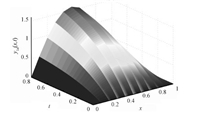
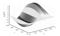
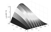
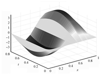
where $(x,t)\in\times[0,0.8]$,the desired trajectories of the iterative learning are $y_{1d}=-2({\rm e}^{-2 t}-1)\sin \pi x$,$y_{2d}=-4\sin \pi t \sin 2 \pi x$,both the initial state value and input value of the control at the beginning of learning are set 0 and $r=0$,then it is easy to calculate $\|(I+G(t)\Gamma(t))^{-1}\|^2<0.5$,then the condition of Theorem 1(or Theorem 2,Theorem 3) is satisfied,the ILC adopted is based on close-loop P-type. By the forward difference method,the simulation results are shown in Figs.1 $\sim$ 7.

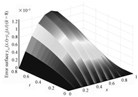
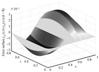
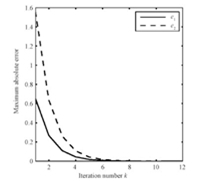
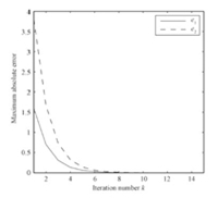
Figs.1 and 2 are the desired curved surfaces,Figs.3 and 4 are relative curved surfaces at the eighth iterations,Figs.5 and 6 are error curved surface. Figs.7 and 8 are the curve charts describing the variation of the maximum tracking error with iteration number by using the close-loop ILC and open-loop ILC,respectively. Numerically,when the number of iterations is eight,the absolute values of the maximum tracking error are $1.269\times10^{-3},3.013\times10^{-3}$ by using close-loop ILC,employing open-loop ILC the absolute values of the maximum tracking error are $5.096\times10^{-3},1.214\times10^{-3}$,respectively. Therefore,Figs.1$\sim$7 show that close loop ILC is effective. Meanwhile,from Figs.7 and 8,we can see that the close-loop ILC is superior to the open-loop ILC for systems (58).

V. CONCLUSION

A class of parabolic distributed parameter systems,with coefficient matrix uncertain but bounded,is studied by using the close-loop P-type iterative learning algorithm. $L^2$-norms and $W^{1,2}$-norms of the tracking error convergence analysis is given without any model simplification or discretization. The theoretical analysis and simulation results show that the close-loop P-type iterative learning algorithm applicable to ordinary differential systems can be extended to distributed parameter systems. We will look for more learning algorithms that can be applied to the distributed parameter systems in the future.