2. School of Information Science and Technology, Dalian Maritime University, Dalian 116026, China;
3. Research Center of Information and Control, Dalian University of Technology, Dalian 116024, China
IN recent years,the problems of sparse signal recovery have been widely investigated because of the emergence of new signal sampling theory which is known as compressed sampling or compressed sensing (CS)[1, 2, 3]. Using less measurements than those required in Shannon sample principle,a sparse signal can be recovered with overwhelming probability by solving a 1-norm minimization problem. This convex optimization problem can be solved by various methods,such as basis pursuit de-noising (BPDN),least absolute shrinkage and selection operator (LASSO), Dantzig selector (DS),etc. Many researchers have attempted to discuss this problem in the classic framework of signal estimation,such as Kalman filtering (KF). In [4],the Dantzig selector was used to estimate the support set of a sparse signal, and then a reduced-order Kalman filter was employed to recover the signal. In [5],the authors presented an algorithm based on a hierarchical probabilistic model that used re-weighted $\ell_1$ minimization as its core computation and propagated second order statistics through time similar to classic Kalman filtering. The dual problem of 1-norm minimization was solved in [6] by introducing a pseudo-measurement equation into Kalman filtering, and the Bayesian interpretation of this method was provided in [7].
Distributed sensor network is an important way of data acquisition in engineering,and the distributed estimation or filtering problems have been paid much attention recently[8, 9, 10]. In [11],three types of distributed Kalman filtering algorithms were proposed. A distributed high-pass consensus filter was used to fuse local sensor measurements,such that all nodes could track the average measurement of the whole network. These algorithms were established based on Kalman filtering in information form, and analysis of stability and performance of Kalman-consensus filter was provided in [12]. It is well known that robustness of Kalman filtering is not satisfactory. In [13],a design method of distributed $H_{\infty}$ filtering for polynomial nonlinear stochastic systems was presented,and the filter parameters were derived in terms of a set of parameter-dependent linear matrix inequalities (PDLMIs) such that a desired $H_{\infty}$ performance was achieved. A $H_{\infty}$-type performance index was established in [14] to measure the disagreement between adjacent nodes,and the distributed robust filtering problem was solved with a vector dissipativity method. Nevertheless,the distributed sparse signal estimation problem has not been adequately researched yet in the framework of $H_{\infty}$ filtering.
In this paper,we aim to combine the pseudo-measurement method with $H_{\infty}$ filtering,and develop a distributed $H_{\infty}$ filtering algorithm to estimate a sparse signal sequence using the measurements distributed over a sensor network. A $\ell_1$-regularized $H_{\infty}$ filter is established at first and the pseudo-measurement equation can be interpreted as a 1-norm regularization term added to the classic $H_{\infty}$ performance index. To develop the distributed algorithm,a high-pass consensus filter is embedded into $\ell_1$-regularized $H_{\infty}$ filter in information form,such that all node filters can reach a consensus on the estimates of sparse signals asymptotically and satisfy the prescribed $H_{\infty}$ performance constraint.
The remainder of this paper is organized as follows. Section Ⅱ gives a brief overview of basic problems in compressed sampling,and introduces the sparse signal recovery method using Kalman filtering with embedded pseudo-measurement. In Section Ⅲ,the centralized $\ell_1$-regularized $H_{\infty}$ filtering method is established by means of Krein space Kalman filtering,and the corresponding information filter is derived. A high-pass consensus filter is employed to develop the distributed filtering algorithm in Section Ⅳ. Simulation results are given in Section V to demonstrate effectiveness of the proposed method,and Section Ⅵ provides some concluding remarks.
Notation. The notation used here is fairly standard except where otherwise stated. The support set of ${\pmb x}\in\mathbf{R}^n$ is defined as ${\rm Supp}\{{\pmb x}\} = \{i | {\pmb x}(i)\neq 0\}$. $\|{\pmb x}\|_0$ is the cardinality of ${\rm Supp}\{{\pmb x}\}$. The 1-norm and 2-norm of ${\pmb x}$ are defined as $\parallel x{\parallel _1} = \sum\nolimits_{i = 1}^n {|x(i)|} $ and $\parallel x{\parallel _2} = \sqrt {{x^{\rm{T}}}x} $,respectively. $x_P^2$ means the product ${x^{\rm{T}}}Px$. ${\rm{sgn}}( \cdot )$ is the sign function. ${\rm{E}}[\xi ]$ defines the mathematical expectation of random variable $\xi $. ${\rm{N}}(\mu ,{\sigma ^2})$ stands for normal distribution with mean $\mu $ and variance ${\sigma ^2}$. ${{\rm{U}}_{{\rm{int}}}}[a,b]$ defines the integer uniform distribution in the interval $[a,b]$. ${\rm{vec}}\{ {x_1}, \cdots ,{x_n}\} : = {\left[ {x_1^{\rm{T}} \cdots x_n^{\rm{T}}} \right]^{\rm{T}}}$. ${\rm{diag}}\{ {A_1}, \cdots ,{A_n}\} $ denotes a block-diagonal matrix whose diagonal blocks are given by ${A_1}, \cdots ,{A_n}$. $S0$ (respectively,$S \succ 0$) means a real symmetric matrix $S$ is positive semi-definite (respectively, positive definite).
Ⅱ. SPARSE SIGNAL ESTIMATION USING KALMAN FILTERINGThis section briefly overviews some basic issues in compressed sampling theory,and introduces the pseudo-measurement embedded Kalman filtering method proposed in [6]. More details can be found in [1, 2, 3, 6, 7].
A. Sparse Signal RecoveryA signal ${\pmb x} \in\mathbf{R}^n$ is sparse if $\|{\pmb x}\|_0\ll n$,and ${\pmb x}$ is called $s$-sparse if $\|{\pmb x}\|_0=s$. Assume $\{{\pmb x}_k\}_{k=0}^{N}$ is an unknown discrete-time sparse signal sequence in $\mathbf{R}^n$ and ${\pmb x}_k$ evolves according to the following dynamic model
| \begin{align} {\pmb x}_{k+1} = A_k {\pmb x}_k + {\pmb w}_k, \end{align} | (1) |
where $A_k \in \mathbf{R}^{n\times n}$ is the state transition matrix,$\{{\pmb w}_k\}_{k=0}^{N-1}$ is a zero-mean white Gaussian sequence with covariance $Q_k \succeq 0$,and ${\pmb x}_0\sim {\rm N}({\pmb x}_{0|-1},P_{0|-1})$. The $m$-dimensional linear measurement of ${\pmb x}_k$ is
| \begin{align} {\pmb y}_k = C_k {\pmb x}_k + {\pmb v}_k, \end{align} | (2) |
where $C_k \in \mathbf{R}^{m\times n}$ is the measurement matrix, and $\{{\pmb v}_k\}_{k=0}^{N}$ is a zero-mean white Gaussian sequence with covariance $R_k \succeq 0$. Extracting signal ${\pmb x}_k$ from measurement ${\pmb y}_k$ is an ill-posed problem in general when $m<n$.
As shown in [1, 2, 3],${\pmb x}_k$ can be accurately recovered by solving the following optimization problem
| \begin{align} \underset{\hat{{\pmb x}}_k \in \mathbf{R}^n}{\min} \|\hat{{\pmb x}}_k\|_0,~~\text{s.t.}~~\|{\pmb y}_k-C_k\hat{{\pmb x}}_k\|_2^2 \leq \varepsilon. \end{align} | (3) |
But the optimization problem (3) is NP-hard and cannot be solved effectively. Fortunately,the authors of [1] have shown that if the measurement matrix $C_k$ obeys the so-called restricted isometry property (RIP),the solution of (3) can be obtained with overwhelming probability by solving the following convex optimization problem
| \begin{align} \underset{\hat{{\pmb x}}_k \in \mathbf{R}^n}{\min} \|\hat{{\pmb x}}_k\|_1,~~\text{s.t.}~~\|{\pmb y}_k-C_k\hat{{\pmb x}}_k\|_2^2 \leq \varepsilon. \end{align} | (4) |
This is a fundamental result in compressive sampling,and one of the deep results is that for a $s$-sparse signal in $\mathbf{ R}^n$,only on the order of $m = s\log n$ samples are needed to reconstruct it.
B. Pseudo-measurement Embedded Kalman FilteringFor the system given in (1) and (2),Kalman filtering can provide an estimate of ${\pmb x}_k$ which is a solution of the following unconstrained $\ell_2$ minimization problem
| \begin{align} \underset{\hat{{\pmb x}}_k \in \mathbf{R}^n}{\min} {\rm E}_{{\pmb x}_k|{\pmb y}_1,\cdots,{\pmb y}_k}\Big[\|{\pmb x}_k-\hat{{\pmb x}}_k\|_2^2\Big]. \end{align} | (5) |
In [6],the authors discussed the stochastic case of (4)
| \begin{align} \underset{\hat{{\pmb x}}_k \in \mathbf{R}^n}{\min} \|\hat{{\pmb x}}_k\|_1,~~\text{s.t.}~~ {\rm E}_{{\pmb x}_k|{\pmb y}_1,\cdots,{\pmb y}_k}\Big[\|{\pmb x}_k-\hat{{\pmb x}}_k\|_2^2\Big] \leq \varepsilon \end{align} | (6) |
and its dual problem
| \begin{align} \underset{\hat{{\pmb x}}_k \in \mathbf{R}^n}{\min} {\rm E}_{{\pmb x}_k|{\pmb y}_1,\cdots,{\pmb y}_k}\Big[\|{\pmb x}_k-\hat{{\pmb x}}_k\|_2^2\Big],~~\text{s.t.}~~\|\hat{{\pmb x}}_k\|_1\leq\varepsilon'. \end{align} | (7) |
By constructing a pseudo-measurement equation
| \begin{align} 0 = H_k{\pmb x}_k-\varepsilon'_k, \end{align} | (8) |
where $H_k = {\rm sgn}({\pmb x}_k^\mathrm{T})$,and $\varepsilon'_k\sim{\rm N}(0,\sigma_k^2)$ serves as the fictitious measurement noise,the constrained optimization problem (7) can be solved in the framework of Kalman filtering and the specific method has been summarized as CS-embedded KF with 1-norm constraint (CSKF-1) algorithm in [6].
In the pseudo-measurement equation (8),the measurement matrix $H_k$ is state-dependent,and it can be approximated by $\hat{H}_k = {\rm sgn}(\hat{{\pmb x}}_{k}^\mathrm{T})$. The divergence of this approximation was discussed in [7]. Furthermore, $\sigma_k$ is a tuneable parameter which determines the tightness of constraint on 1-norm of the state estimate $\hat{{\pmb x}}_k$.
Ⅲ. $\pmb {\ell_1}$-REGULARIZED $\pmb {H_{\infty}}$ FILTERINGIn this section,the pseudo-measurement equation is combined with $H_{\infty}$ filtering,and a $\ell_1$-regularized $H_{\infty}$ filtering is developed for estimating a sparse signal sequence.
Define the augmented measurement equation using (2) and (8) as
| \begin{align} \bar{{\pmb y}}_k = \bar{C}_k{\pmb x}_k + \bar{{\pmb v}}_k, \end{align} | (9) |
where $\bar{{\pmb y}}_k=\left[ \begin{array}{c} {\pmb y}_k \\ 0 \\ \end{array} \right]$, $\bar{C}_k = \left[ \begin{array}{c} C_k \\ H_k \\ \end{array} \right]$, $\bar{{\pmb v}}_k = \left[ \begin{array}{c} {\pmb v}_k \\ \varepsilon'_k \\ \end{array} \right]$, and denote $\bar{R}_k = \left[ \begin{array}{cc} R_k & 0 \\ 0 & \sigma_k^2 \\ \end{array} \right]$. Consider the system described by (1) and (9) with Gramian matrix
| \begin{align} \Bigg\langle\left[ \begin{array}{c} {\pmb x}_0 \\ {\pmb w}_k \\ \bar{{\pmb v}}_k \\ \end{array} \right], \left[ \begin{array}{c} {\pmb x}_0 \\ {\pmb w}_j \\ \bar{{\pmb v}}_j \\ \end{array} \right] \Bigg\rangle = \left[ \begin{array}{ccc} P_{0|-1} & 0 & 0 \\ 0 & Q_k\delta_{kj} & 0 \\ 0 & 0 & \bar{R}_k\delta_{kj} \\ \end{array} \right], \end{align} | (10) |
where $\delta_{kj}$ is Kronecker delta function. We aim to design a full-order filter in the form of
| \begin{align} \hat{{\pmb x}}_k = A_{k-1}\hat{{\pmb x}}_{k-1} + K_k(\bar{{\pmb y}}_k-\bar{C}_kA_{k-1}\hat{{\pmb x}}_{k-1}), \end{align} | (11) |
such that for all non-zero ${\pmb w}_k$ and ${\pmb v}_k$,the filtering error $\tilde{{\pmb x}}_k={\pmb x}_k-\hat{{\pmb x}}_k$ satisfies the following $\ell_1$-regularized $H_{\infty}$ performance constraint
| \begin{align} &\sum_{k=0}^N\|\tilde{{\pmb x}}_k\|_2^2 < \gamma^2\Bigg( \|{\pmb x}_0-{\pmb x}_{0|-1}\|_{P_{0|-1}^{-1}}^2+ \sum_{k=0}^{N-1}\|{\pmb w}_k\|_{Q_k^{-1}}^2 +\nonumber\\ &\quad \sum_{k=0}^{N}\|{\pmb v}_k\|_{R_k^{-1}}^2+\sum_{k=0}^{N}\sigma_k^{-2}\|{\pmb x}_k\|_1^2\Bigg), \end{align} | (12) |
where $\gamma>0$ is a prescribed scalar.
There exists a filter in the form of (11) achieving the performance (12),if and only if the filtering error covariance matrix $P_{k|k}$ satisfies
| \begin{align} P_{k|k}^{-1} = P_{k|k-1}^{-1}+C_k^\mathrm{T}R_k^{-1}C_k + \sigma_k^{-2}H_k^\mathrm{T}H_k-\gamma^{-2}I \succ 0, \end{align} | (13) |
for $0\leq k < N$,where the initial value is $P_{0|-1}$,and the predicted error covariance matrix $P_{k|k-1}$ satisfies the Riccati recursion
| \begin{align} P_{k|k-1} = A_{k-1}P_{k-1|k-1}A_{k-1}^\mathrm{T}+Q_{k-1}. \end{align} | (14) |
The filtered estimates $\hat{{\pmb x}}_{k|k}$ are recursively computed as
| \begin{align} \hat{{\pmb x}}_{k|k} = \hat{{\pmb x}}_{k|k-1} + K_k(\bar{{\pmb y}}_k-\bar{C}_k\hat{{\pmb x}}_{k|k-1}), \end{align} | (15) |
where
| \begin{align} K_k = P_{k|k-1}\bar{C}_k^\mathrm{T}(\bar{C}_kP_{k|k-1}\bar{C}_k^\mathrm{T}+\bar{R}_k)^{-1}, \end{align} | (16) |
and the predicted estimates
| \begin{align} \hat{{\pmb x}}_{k|k-1} = A_{k-1}\hat{{\pmb x}}_{k-1|k-1}. \end{align} | (17) |
Proof. Define the quadratic performance function
| \begin{align*} &J_{\infty} = \|{\pmb x}_0-{\pmb x}_{0|-1}\|_{P_{0|-1}^{-1}}^2 + \sum_{k=0}^{N-1}\|{\pmb w}_k\|_{Q_k^{-1}}^2 + \sum_{k=0}^{N}\|{\pmb v}_k\|_{R_k^{-1}}^2+ \\ &\quad \sum_{k=0}^{N}\sigma_k^{-2}\|{\pmb x}_k\|_1^2- \gamma^{-2}\sum_{k=0}^N\|\tilde{{\pmb x}}_k\|_2^2=\\ &\quad \|{\pmb x}_0-{\pmb x}_{0|-1}\|_{P_{0|-1}^{-1}}^2 + \sum_{k=0}^{N-1}\|{\pmb w}_k\|_{Q_k^{-1}}^2 +\\ &\quad \sum_{k=0}^N\|\breve{{\pmb y}}-\breve{C}{\pmb x}_k\|_{\breve{R}_k^{-1}}^2, \end{align*} |
where $\breve{{\pmb y}}_k=\left[ \begin{array}{c} {\pmb y}_k \\ 0 \\ \hat{{\pmb x}}_{k|k} \\ \end{array} \right]$, $\breve{C}_k=\left[ \begin{array}{c} C_k \\ H_k \\ I \\ \end{array} \right]$ and $\breve{R}_k=\left[ \begin{array}{ccc} R_k & 0 & 0 \\ 0 & \sigma_k^2 & 0 \\ 0 & 0 &-\gamma^2I \\ \end{array} \right]$. Then the proposed filter is not hard to obtain according to Krein space Kalman filtering in [15]. Details of the proof are omitted.
In [7],the pseudo-measurement equation (8) was interpreted in Bayesian filtering framework,and a semi-Gaussian prior distribution was discussed. Here,according to Theorem 1,the pseudo-measurement equation in $H_{\infty}$ filtering can be interpreted as a 1-norm regularization term added to the classic $H_{\infty}$ performance index.
To establish a distributed filtering algorithm,the result in Theorem 1 will be rebuilt in information form,so by denoting
| \begin{align} &{\pmb z}_k = {{\bar C}_k}^\mathrm{T}{{\bar R}}_k^{-1}{\bar {\pmb y}}_k=C_k^\mathrm{T}R_k^{-1}{\pmb y}_k,\end{align} | (18) |
| \begin{align} &S^[1]_k = C_k^\mathrm{T}R_{k}^{-1}C_k ,\end{align} | (19) |
| \begin{align} &S^[2]_k = \sigma_k^{-2}H_k^\mathrm{T}H_k, \end{align} | (20) |
we can obtain the $\ell_1$-regularized $H_{\infty}$ information filter.
The filter established in Theorem 1 is equivalent to the following information form.
Measurement update:
| \begin{align} &\hat{P}_{k|k}^{-1} = P_{k|k-1}^{-1}+S^[1]_k,\end{align} | (21) |
| \begin{align} &\hat{{\pmb x}}_{k|k}^-= \hat{{\pmb x}}_{k|k-1}+\hat{P}_{k|k}({\pmb z}_k-S^[1]_k\hat{{\pmb x}}_{k|k-1}). \end{align} | (22) |
Pseudo-measurement update:
| \begin{align} &P_{k|k}^{-1} = \hat{P}_{k|k}^{-1}+S^[2]_k-\gamma^{-2}I,\end{align} | (23) |
| \begin{align} &\hat{{\pmb x}}_{k|k} = \Big(I-(P_{k|k}^{-1}+\gamma^{-2}I)^{-1}S^[2]_k\Big)\hat{{\pmb x}}_{k|k}^-. \end{align} | (24) |
Time update:
| \begin{align} &P_{k+1|k} = A_kP_{k|k}A_k^\mathrm{T} + Q_k,\end{align} | (25) |
| \begin{align}&\hat{{\pmb x}}_{k+1|k} = A_k\hat{{\pmb x}}_{k|k}. \end{align} | (26) |
Proof. According to matrix inversion lemma,we have
| \begin{align*} &K_k = P_{k|k-1}\bar{C}_k^\mathrm{T}(\bar{C}_kP_{k|k-1}\bar{C}_k^\mathrm{T}+\bar{R}_k)^{-1} =\\ &\quad(P_{k|k-1}^{-1}+\bar{C}_k^\mathrm{T}\bar{R}_k^{-1}\bar{C}_k^\mathrm{T})^{-1}\bar{C}_k^\mathrm{T}\bar{R}_k^{-1} =\\ &\quad (P_{k|k}^{-1}+\gamma^{-2}I)^{-1}\bar{C}_k^\mathrm{T}\bar{R}_k^{-1}, \end{align*} |
then (15) can be rewritten as
| \begin{align*} &\hat{{\pmb x}}_{k|k} = \hat{{\pmb x}}_{k|k-1}+(P_{k|k}^{-1}+\gamma^{-2}I)^{-1}\times\\ &\quad \Big({\pmb z}_k- (S^[1]_k+S^[2]_k)\hat{{\pmb x}}_{k|k-1}\Big)= \\ &\quad \Big(I-(P_{k|k}^{-1}+\gamma^{-2}I)^{-1}S^[2]_k\Big)\hat{{\pmb x}}_{k|k-1} +\\ &\quad (P_{k|k}^{-1}+\gamma^{-2}I)^{-1}\Big({\pmb z}_k- S^[1]_k\hat{{\pmb x}}_{k|k-1}\Big). \end{align*} |
On the other hand,by substituting (22) into (24),we have
| \begin{align*} &\hat{{\pmb x}}_{k|k} = \Big(I-(P_{k|k}^{-1}+\gamma^{-2}I)^{-1}S^[2]_k\Big)\times\\ &\quad \Big(\hat{{\pmb x}}_{k|k-1}+\hat{P}_{k|k}({\pmb z}_k-S^[1]_k\hat{{\pmb x}}_{k|k-1})\Big)=\\ &\quad \Big(I-(P_{k|k}^{-1}+\gamma^{-2}I)^{-1}S^[2]_k\Big)\hat{{\pmb x}}_{k|k-1}+\\ &\quad \Big(I-(P_{k|k}^{-1}+\gamma^{-2}I)^{-1}S^[2]_k\Big) \hat{P}_{k|k}\Big({\pmb z}_k-S^[1]_k\hat{{\pmb x}}_{k|k-1}\Big). \end{align*} |
It is easy to obtain the following equation
| \begin{align*} &\hat{P}_{k|k}^{-1}\Big(I-(P_{k|k}^{-1}+\gamma^{-2}I)^{-1}S^[2]_k\Big)^{-1}=\\ &\quad \hat{P}_{k|k}^{-1}\Big(I-(S^[2]_k-P_{k|k}^{-1}-\gamma^{-2}I)^{-1}S^[2]_k\Big) =\\ &\quad \hat{P}_{k|k}^{-1}\Big(I+\hat{P}_{k|k}S^[2]_k\Big) =&\\ &\quad P_{k|k}^{-1}+\gamma^{-2}I, \end{align*} |
so
| \begin{align*} \Big(P_{k|k}^{-1}+\gamma^{-2}I\Big)^{-1} = \Big(I-(P_{k|k}^{-1}+\gamma^{-2}I)^{-1}S^[2]_k\Big)\hat{P}_{k|k}, \end{align*} |
which means (15) is equivalent to (22) and (24). Equation (13) is obtained immediately by combining (21) and (23).
Ⅳ. DISTRIBUTED $\pmb {H_{\infty}}$-CONSENSUS FILTERING WITH PSEUDO-MEASUREMENTIn this section,we will develop a distributed $H_{\infty}$-consensus filtering based on the results presented in Section Ⅲ.
Consider a sensor network whose topology is represented by an undirected graph $\mathcal{G}=(\mathcal{V,E,A})$ of order $r$ with the set of nodes $\mathcal{V}=\{1,2,\cdots,r\}$,the set of edges $\mathcal{E} \subseteq \mathcal{V}\times\mathcal{V}$,and the adjacency matrix $\mathcal{A}=[a_{ij}]_{r\times r}$ with nonnegative adjacency elements $a_{ij}$. An edge of $\mathcal{G}$ is denoted by an unordered pair $(i,j)$. The adjacency elements associated with the edges are positive,i.e., $a_{ij}>0\Leftrightarrow (i,j)\in \mathcal{E}$. Node $j$ is called a neighbor of node $i$ if $(i,j)\in \mathcal{E}$ and $j\neq i$. The neighbor set of node $i$ is denoted by $\mathcal{N}_i$. Assume $\mathcal{G}$ is strongly connected.
Assume the measurement of sensor node $i$ is described by the linear model (2). Denote $\bar{{\pmb y}}_{i,k}=\left[ \begin{array}{c} {\pmb y}_{i,k} \\ 0 \\ \end{array} \right]$, $\bar{C}_{i,k}=\left[ \begin{array}{c} C_{i,k} \\ H_{k} \\ \end{array} \right]$, $\bar{{\pmb v}}_{i,k}=\left[ \begin{array}{c} {\pmb v}_{i,k} \\ \varepsilon'_{i,k} \\ \end{array} \right]$, we can get the following augmented measurement equation of sensor $i$
| \begin{align} \bar{{\pmb y}}_{i,k} = \bar{C}_{i,k} {\pmb x}_k + \bar{{\pmb v}}_{i,k}, \end{align} | (27) |
where $C_{i,k}$ is the measurement matrix of sensor $i$,$H_{k} = {\rm sgn}({\pmb x}_k^\mathrm{T})$,${\pmb v}_{i,k}\sim{\rm N}(0,R_{i,k})$,$\varepsilon'_{i,k}\sim{\rm N}(0,\sigma_{i,k}^2)$. And let $\bar{R}_{i,k}={\rm diag}\{R_{i,k},\sigma_{i,k}^2\}$. Define $\mathcal{Y}_k = {\rm vec}\{\bar{{\pmb y}}_{1,k},\cdots,\bar{{\pmb y}}_{r,k}\}$,$\mathcal{V}_k = {\rm vec}\{\bar{{\pmb v}}_{1,k},\cdots,\bar{{\pmb v}}_{r,k}\}$, $\mathcal{C}_k = {\rm vec}\{\bar{C}_{1,k},\cdots,\bar{C}_{r,k}\}$ and ${\mathcal{R}_k} = {\rm diag}\{\bar{R}_{1,k},\cdots,\bar{R}_{r,k}\}$. Then we have the augmented global measurement
| \begin{align} \mathcal{Y}_k = \mathcal{C}_k {\pmb x}_k + \mathcal{V}_k. \end{align} | (28) |
Denoting
| \begin{align} {\pmb z}_k=\frac{1}{r}\sum_{i=1}^r\bar{C}_{i,k}^\mathrm{T}\bar{R}_{i,k}^{-1}\bar{{\pmb y}}_{i,k}=\frac{1}{r}\sum_{i=1}^rC_{i,k}R_{i,k}^{-1}{\pmb y}_{i,k}, \end{align} | (29) |
| \begin{align} \bar{S}_k=\frac{1}{r}\sum_{i=1}^r\bar{C}_{i,k}^\mathrm{T}\bar{R}_{i,k}^{-1}\bar{C}_{i,k} :=\bar{S}^[1]_{k}+\bar{S}^[2]_{k}, \end{align} | (30) |
where $\bar{S}^[1]_{k}=\frac{1}{r}\sum_{i=1}^rC_{i,k}^\mathrm{T}R_{i,k}^{-1}C_{i,k}$ and $\bar{S}^[2]_{k}=\frac{1}{r}\sum_{i=1}^r\sigma_{i,k}^{-2}H_k^\mathrm{T}H_k$, we can obtain a local filter for each sensor node,which has the same performance as the centralized filter presented in Theorem 1 by using the augmented global measurement (28).
Suppose every node of the network applies the following filter
| \begin{align*} &\hat{P}_{i,k|k}^{-1} = P_{i,k|k-1}^{-1}+\bar{S}^[1]_k,\\ &\hat{{\pmb x}}_{i,k|k}^-= \hat{{\pmb x}}_{i,k|k-1}+\hat{P}_{i,k|k}({\pmb z}_k-\bar{S}^[1]_k\hat{{\pmb x}}_{i,k|k-1}),\\ &P_{i,k|k}^{-1} = \hat{P}_{i,k|k}^{-1}+\bar{S}^[2]_k-\gamma^{-2}I,\\ &\hat{{\pmb x}}_{i,k|k} = \Big(I-(P_{i,k|k}^{-1}+\gamma^{-2}I)^{-1}\bar{S}^[2]_k\Big)\hat{{\pmb x}}_{i,k|k}^-,\\ &P_{i,k+1|k} = A_kP_{i,k|k}A_k^\mathrm{T} + rQ_k,~~~~~~~~~~~~~~~ \\ &\hat{{\pmb x}}_{i,k+1|k} = A_k\hat{{\pmb x}}_{i,k|k}, \end{align*} |
where $P_{i,0|-1}=rP_{0|-1}$,then the local and central state estimates for all nodes are the same,i.e.,$\hat{{\pmb x}}_{i,k|k}=\hat{{\pmb x}}_{k|k}$.
Proof. The proof is a direct combination of Corollary 1 and the result in [11].
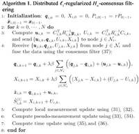
In Corollary 2,the average measurement ${\pmb z}_k$ and the average inverse covariance matrix $\bar S_k^{^{\left[ 1 \right]}}$ can be computed approximately on each node using the following high-pass consensus filter proposed in [11]
| \begin{align} \left\{ \begin{array}{rcl} \dot{{\pmb q}}_i&=&\beta\sum_{j \in \mathcal{N}_i}\Big(({\pmb q}_j-{\pmb q}_i)+({\pmb u}_j-{\pmb u}_i)\Big),~~~\beta > 0,\\ {\pmb \xi}_i &=& {\pmb q}_i + {\pmb u}_i. \end{array} \right. \end{align} | (31) |
It has been verified that,if the network is strongly connected, ${\pmb \xi}_i\rightarrow \frac{1}{r}\sum_{i=1}^r{\pmb u}_i$ as $t\rightarrow\infty$ for any $i \in \mathcal{V}$. $\bar S_k^{^{\left[ 2 \right]}}$ can be approximated on each node by $\bar S_{i,k}^{^{\left[ 2 \right]}}=\sigma_{i,k}^{-2}\hat{H}_{i,k}^\mathrm{T}\hat{H}_{i,k}$, where $\hat{H}_{i,k} = {\rm sgn}(\hat{{\pmb x}}_{i,k|k}^-)^\mathrm{T}.$p>
The distributed $H_{\infty}$ filtering can be summarized as the following Algorithm 1.
|
Download:
|
In this section,we will illustrate effectiveness of the method proposed in Section Ⅳ.
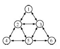
Without loss of generality,consider a sensor network with 6 nodes as shown in Fig. 1,whose topology is represented by an undirected graph $\mathcal{G}=(\mathcal {V},\mathcal {E}, \mathcal {A})$ with the set of nodes $\mathcal{V}=\{1,2,3,4,5,6\}$,the set of edges $\mathcal{E}=\{(1,1),(1,2),(1,3),(2,2),(2,3),(2,4),(2,5),(3,3),(3,5),(3,6),$ $(4,4),(4,5),(5,5),(5,6),(6,6)\}$,and the adjacency matrix
| \begin{align*} \mathcal {A}=\left[ \begin{array}{cccccc} 1 & 1 & 1 & 0 & 0 & 0 \\ 1 & 1 & 1 & 1 & 1 & 0 \\ 1 & 1 & 1 & 0 & 1 & 1 \\ 0 & 1 & 0 & 1 & 1 & 0 \\ 0 & 1 & 1 & 1 & 1 & 1 \\ 0 & 0 & 1 & 0 & 1 & 1 \\ \end{array} \right]. \end{align*} |
|
Download:
|
| Fig. 1. Topological structure of the sensor network. | |
Here,we attempt to estimate a 10-sparse signal sequence $\{{\pmb x}_k\}$ in $\mathbf{R}^{256}$ and assume the sequence has a constant support set. The dynamics of $\{{\pmb x}_k\}$ can be described by the following linear system
| \begin{align} {\pmb x}_{k+1}(i)= \left\{ \begin{array}{ccl} {\pmb x}_{k}(i)+{\pmb w}_{k}(i),&~& i \in {\rm Supp}\{{\pmb x}_0\},\\ 0,&~& \text{otherwise}, \end{array} \right. \end{align} | (32) |
where $\{{\pmb w}_{k}(i)\}$ is a zero-mean Gaussian white noise sequence with standard deviation 0.01. For system (1),we have $A = I_{256}$ and $Q_k = 10^{-4} \times I_{256}$. Both the index $i \in {\rm Supp}\{{\pmb x}_k\}$ and the value of ${\pmb x}_k(i)$ are unknown. The initial sparse signal ${\pmb x}_0$ is generated by creating the support set as $i\sim {\rm U}_\mathrm{int}[1, 256]$ and setting the value as ${\pmb x}_0(i)\sim {\rm N}(0,1)$. For sensor node $i$,the sensing matrix $C_{i,k} \in \mathbf{R}^{12\times 256}$ consists of entries sampled according to ${\rm N}(0,\frac{1}{72})$. Then,we have the global measurement ${\pmb y}_{\mathrm{cent}} = {\rm vec}\{{\pmb y}_1,\cdots,{\pmb y}_6\} \in \mathbf{R}^{72}$
|
|
Table I NMSEs WHEN $k=80$ |
and the global measurement matrix $C_{\mathrm{cent}} = {\rm vec}\{C_1,\cdots,\\C_6\} \in \mathbf{R}^{72\times 256}$. This type of matrix like $C_{\mathrm{cent}}$ has been shown to satisfy the restricted isometry property with overwhelming probability. The measurement noise ${\pmb v}_{i,k} \sim {\rm N}(0,R_{i,k})$, where $R_{i,k}=10^{-4} \times I_{12}$,and denote $R_{\mathrm{cent}} = {\rm diag}\{R_1,\cdots,R_6\}\in \mathbf{R}^{72\times 72}$. Set filter initial states as $\hat{{\pmb x}}_{i,0|-1}=0~(i = 1,\cdots,6)$,and filter parameters as $\beta=0.2$,$\lambda=1$,$\gamma=10$,$\sigma_{i,k} = 10+0.5k$,and $N=80$.
Now we are ready to design the distributed $H_{\infty}$ filters for system (38). The centralized Kalman filtering and CSKF-1 algorithm proposed in [6] are implemented respectively using ${\pmb y}_{\mathrm{cent}}$,$C_{\mathrm{cent}}$ and $R_{\mathrm{cent}}$,and we will compare their performances with that of Algorithm 1. The following normalized mean squared error (NMSE) is employed to evaluate the performance,
| \begin{align*} { e} = \frac{\|{\pmb x}-\hat{{\pmb x}}\|_2^2}{\|{\pmb x}\|_2^2}. \end{align*} |
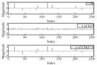
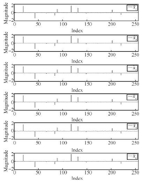
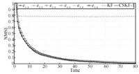
The results are presented in Figs. 2$\sim$4. In Fig. 2,the first figure shows the actual signal ${\pmb x}_{80}$,the second figure gives $\hat{{\pmb x}}_{80}$ from centralized Kalman filtering,the third figure shows $\hat{{\pmb x}}_{80}$ from centralized CSKF-1 algorithm. Fig. 3 gives the estimates of ${\pmb x}_{80}$ from sensor nodes using Algorithm 1. It is obvious that all nodes give satisfactory estimates of the actual sparse signal. Fig. 4 presents the normalized mean squared errors,which indicates that all node filters are stable and reach a consensus on the estimates of sparse signals. Moreover,there exist smaller steady errors by using Algorithm 1 than centralized Kalman filtering and CSKF-1 algorithm, and the errors when $k=80$ are presented in Table I. All of these results demonstrate effectiveness of the distributed filter presented in this paper.
|
Download:
|
| Fig. 2. Actual signal ${\pmb x}_{80}$ and its estimates $\hat{{\pmb x}}_{80}$ using centralized KF and CSKF-1. | |
In this paper,the problem of distributed sparse signal estimation in sensor networks has been considered. The pseudo-measurement equation was interpreted as a 1-norm regularization term in the classic $H_{\infty}$ performance index,and the $\ell_1$-regularized $H_{\infty}$ filtering method was proposed. By means of a high-pass consensus filter,the distributed $H_{\infty}$ filtering algorithm was established. A numerical example verified effectiveness of the proposed method. However, the algorithm presented in this paper is only suitable to deal with the time-varying sparse signal with an invariant or slowly changing support set,and the more general methods need to combine a support set estimator with the filter. The decomposition of sensing matrix needs further research as well. These problems will be discussed in future work.
|
Download:
|
| Fig. 3. Estimates of ${\pmb x}_{80}$ using Algorithm 1. | |
|
Download:
|
| Fig. 4. MSEs of centralized KF,CSKF-1 and Algorithm 1. | |
| [1] | Candes E J, Romberg J, Tao T. Robust uncertainty principles:exact signal reconstruction from highly incomplete frequency information. IEEE Transactions on Information Theory, 2006, 52(2):489-509 |
| [2] | Candes E J, Romberg J, Tao T. Stable signal recovery from incomplete and inaccurate measurements. Communications on Pure and Applied Mathematics, 2006, 59(8):1207-1223 |
| [3] | Candes E J, Wakin M B. An introduction to compressive sampling. IEEE Signal Processing Magazine, 2008, 25(2):21-30 |
| [4] | Vaswani D. Kalman filtered compressed sensing. In:Proceedings of the 15th IEEE International Conference on Image Processing. San Diego, USA:IEEE, 2008. 893-896 |
| [5] | Charles A S, Rozell C J. Dynamic filtering of sparse signals using reweighted l1. In:Proceedings of the 38th International Conference on Acoustics, Speech, and Signal Processing. Vancouver, Canada:IEEE, 2013. 1-5 |
| [6] | Carmi A, Gurfil P, Kanevsky D. Methods for sparse signal recovery using Kalman filtering with embedded pseudo-measurement norms and quasi-norms. IEEE Transactions on Signal Processing, 2010, 58(4):2405-2409 |
| [7] | Kanevsky D, Carmi A, Horesh L. Kalman filtering for compressed sensing. In:Proceedings of the 13th Conference on Information Fusion (FUSION). Edinburgh, UK:IEEE, 2010. 1-8 |
| [8] | Wan Yi-Ming, Dong Wei, Ye Hao. Distributed H∞ filtering with consensus strategies in sensor networks:considering consensus tracking error. Acat Automatica Sinica, 2012, 38(7):1211-1217(in Chinese) |
| [9] | Wang Shuai, Yang Wen, Shi Hong-Bo. Consensus-based filtering algorithm with packet-dropping. Acat Automatica Sinica, 2010, 36(12):1689-1696(in Chinese) |
| [10] | Feng Xiao-Liang, Wen Cheng-Lin, Liu Wei-Feng, Li Xiao-Fang, Xu Li-Zhong. Sequential fusion finite horizon H∞ filtering for Multisenor System. Acat Automatica Sinica, 2013, 39(9):1523-1532(in Chinese) |
| [11] | Olfati-Saber R. Distributed Kalman filter in sensor networks. In:Proceedings of the 46th IEEE Conference on Decision and Control. Los Angeles, New Orleans, LA:IEEE, 2007. 5492-5498 |
| [12] | Olfati-Saber R. Kalman-consensus filter:optimality, stability, and performance. In:Joint 48th IEEE Conference on Decision and Control and 28th Chinese Control Conference. Shanghai, China:IEEE, 2009. 7036-7042 |
| [13] | Shen B, Wang Z D, Hung Y S, Chesi G. Distributed H∞ filtering for polynomial nonlinear stochastic systems in sensor networks. IEEE Transactions on Industrial Electronics, 2011, 58(5):1971-1979 |
| [14] | Ugrinovskii V. Distributed robust filtering with H∞ consensus of estimates. Automatica, 2011, 47(1):1-13 |
| [15] | Hassibi B, Sayed A H, Kailath T. Indefinite Quadratic Estimation and Control:a Unified Approach to H2 and H∞ Theories. Philadelphia:SIAM, 1999. |
 2014, Vol.1


