 2014, Vol.1


2. School of Information Science and Engineering, Central South University, Changsha 410083, China;
3. School of Information Science and Engineering, Central South University, Changsha 410083, China;
4. School of Automation, China University of Geosciences, Wuhan 430074, China;
5. School of Information Science and Engineering, Central South University, Changsha 410083, China
R EINFORCEMENT learning (RL) is a paradigm of machine learning (ML) in which rewards and punishments guide the learning process. The central idea is learning by interactions with the environment so that the agents can be led to a better state. It is viewed as an effective way to solve strategy optimization for multiple agents[1],and is widely applied in multi-agent systems (MASs),such as the control of robots[2, 3],preventing traffic jams[4],air traffic flow management[5],as well as optimization of production[6]. We particularly focus on the learning algorithms in cooperative multi-agent RL (MARL).
There are lots of papers discussing the challenges in MARL,such as "the curse of dimensionality",nonstationarity,the exploration-exploitation tradeoff,and communication and coordination[7]. Nonstationarity caused by simultaneous learning was concerned mostly in the last decade. The presence of multiple concurrent learners makes the environment non-stationary from a single agent perspective,which is a commonly cited cause of difficulties in MASs,so that the environment is not longer Markovian[8, 9]. Besides,a fundamental issue faced by agents working together is how to efficiently coordinate their own results with a coherent joint behavior[10].
As the size of state-action space quickly becomes too large for classical RL[11],we investigate the case that agents which learn their own behavior in a decentralized way. One of the earliest algorithms applied to decentralized multi-agent environments is Q-learning for independent learners (ILs)[12]. In decentralized Q-learning,no coordination problems are explicitly addressed. Except policy search[13], greedy in the limit with infinite exploration (GLIE)[14], such as $\varepsilon$-greedy or Boltzmann distribution,is a popular single-agent method that decreases the exploration frequency over time so that each agent converges to a constant policy. Besides ILs,various decentralized RL algorithms have been reported in the literature for MAS. In this framework,most authors focus on learning algorithms in fully cooperative MAS. In such environments,the agents share common interests and the same reward function,the individual satisfaction is also the satisfaction of the group[15]. The win-or-learn fast policy hill climbing (WoLF-PHC) algorithm works by applying the win-or-learn fast (WoLF) principle to the policy hill climbing (PHC) algorithm[16],in which agents' strategies are saved as Q-table. Frequency maximum Q-value (FMQ)[17] works only on the repeated game,in which the Q-value of an action in the Boltzmann exploration strategy is changed by a heuristic value. Hysteretic Q-learning[18] is proposed to avoid the overestimation Q-value in stochastic games.
In order to develop a coordinate mechanism for decentralized learning,while avoiding non-stationary induced by simultaneous learning,we concentrate on a popular scenario of MARL,where the agents share common interests and the same reward function. We propose a decentralized RL algorithm,based on which we develop a learning framework for cooperative policy learning. The definition of even discounted reward (EDR) is proposed firstly. Then,we propose a new learning framework,timesharing-tracking framework (TTF),in order to improve EDR to get the optimal cooperative policy. Unlike some aforementioned works,the state space is split into many one states in TTF. There is only one learning agent in a certain state,while the learning agents may not be the same in different states. From the perspective of the whole state space, all agents are entitled to learning simultaneously. Next,the best-response Q-learning (BRQ-learning) is proposed to make the agents alternatively learn. The improvement of EDR with TTF has been verified,and a practical algorithm,BRQ-learning with timesharing-tracking (BRQL-TT) is completely built with the proposed switching principle.
The remainder of this paper is organized as follows. In Section Ⅱ, TTF will be proposed and BRQ-learning will be given,and the performance of TTF with BRQ-learning will be discussed. The switching principle of TTF will be proposed to complete TTF in Section Ⅲ. In Section Ⅳ,we will test our algorithm with experiments,and finally draw the conclusions in Section Ⅴ.
Ⅱ. TTF FOR MARLFirstly,some denotations involved in the paper are introduced as follows. Discrete joint state combining agent 1 to $N$ is denoted by ${\pmb s} = [{s^1},{s^2},\cdots ,{s^N}]$,and discrete joint action executed by agent 1 to agent $N$ is denoted by ${\pmb a}=[a^1,a^2,\cdots,a^N]$. The transition probability of joint state ${\pmb s}$ being transited to joint state ${\pmb s'}$ as the joint action ${\pmb a}$ is executed is denoted by $p({\pmb s'}|{\pmb s},{\pmb a})$,and the policy of agent $i$ at joint state ${\pmb s}$,i.e.,the probability of action $a^i$ being selected by agent $i$,is $\pi(a^i|{\pmb s})$. The immediate global reward w.r.t. joint-state-joint-action is $r({\pmb s},{\pmb a})$.
In practice,agents in the cooperative MAS always act as a group, so that the following assumptions are reasonable and will serve as the foundations for the decentralized learning method. And we address this system in this context,namely repeated game.
Assumption 1. Agents have common interests. In common interest games,the agents' rewards are drawn from the same distribution.
Assumption 2. As a group,agents are always able to observe the others' state transitions,which means joint state of MAS is observable.
One of the critical challenges is introducing credit assignment, in order to divide payoff w.r.t. individual agents. But for the fully cooperative MAS,all agents receive the same rewards shown as Assumption 1.
Even if agents are able to get the others' time-varying policies by Assumption 2,concurrent learning is still regarded as a major problem,because the transition of states w.r.t. individuals is unstable. Thus the model-free learning based on stochastic approximation,which is widely used in reinforcement learning,can hardly ensure convergence theoretically,although many experiments show its feasibility in decentralized learning.
This is the basic motivation to optimize the cooperative policy. However,there are some key issues to be solved. The first is the definition of common value function $V$,which describes effects brought by agent actions. Another problem seems more critical that the value of $V$ is unknown before optimization. Thus the cooperative optimization consists of two parts simultaneously,the learning of value function and policy searching which are coupled compactly,because the results of policy searching may change the actual value function during learning,and vice versa.
The well-defined value function is the key to cooperative learning. To develop it,we first introduce the immediate reward of learning agent based on payoff which is fed back from the environment.
Definition 1. The expected immediate reward (EIR) $r({\pmb s},a^i)$ w.r.t. agent $i$ is defined as
| $r(s,{a^i}) = \sum\limits_{{a^1}} \cdots \sum\limits_{{a^{i-1}}} {\sum\limits_{{a^{i + 1}}} { \cdots \sum\limits_{{a^N}} {\prod\limits_{j = 1,j \ne i}^N {\pi _{\rm{*}}^j} ({a^j}|s)r(s,a)} } } ,$ | (1) |
where $a^{i}\in A^{i}$,and $A^i$ is the set of available actions w.r.t. agent $i$.
Let the denotation$\sum\limits\pi_*^{(1,\cdots,N)}(a^{(1,\cdots,N)}|{\pmb s})$ represent $\sum\limits_{a^1}\cdots \sum\limits_{a^{N}}\prod\limits_{j=1}^N \pi_*^j(a^j|{\pmb s})$ for short. Thus,$r({\pmb s},{a^i}) = \sum\limits \pi_*^{(1,\cdots,i-1,i+1,\cdots,N)}(a^{(1,\cdots,i-1,i+1,\cdots,N)}|{\pmb s})r({\pmb s},{\pmb a})$,abbreviated as $r({\pmb s},{a^i}) = \sum\limits_{a^{-i}} \pi_*^{-i}(a^{-i}|{\pmb s})r({\pmb s},{\pmb a})$. To satisfy Assumption 1,all agents learn with a GLIE strategy to converge to the pure policy,in which all the agents have the same reward as the global reward $r({\pmb s},{\pmb a})$.
Based on EIR,a common expectation of infinite discounted reward for all agents is then developed.
Definition 2. The even discounted reward (EDR) is defined as
| ${V_*}({\pmb s})=\lim\limits_{L \to \infty }{\rm E}\left (\sum_{t=0}^{L}\gamma^{t}\sum\limits_{{\pmb a}}\pi_*({\pmb a}| {\pmb s}_t)r({\pmb s}_t,{\pmb a})|{\pmb s}_{0}={\pmb s}\right ),$ | (2) |
where $\gamma \in$ [0,1) is the discounted factor,and ${\sum \limits_{\pmb a}}\pi_*({\pmb a}| {\pmb s}_{t})r({\pmb s}_{t},{\pmb a})$ represents the item $\sum\limits_{a^1}\sum\limits_{a^2}\cdots\sum\limits_{a^N}\prod\limits_{i=1}^N \pi_*(a^i| {\pmb s}_{t})$ $r({\pmb s}_{t},{\pmb a})$ for short.
It is easy to find the relationship between EIR and EDR w.r.t. agent $i$ as
| $\begin{array}{l} {V_*}\left( s \right) = \mathop {\lim }\limits_{L \to \infty } {\rm{E}}\left( {\sum\limits_{t = 0}^L {{\gamma ^t}} \sum\limits_{{a^i}} {\pi _*^i} \left( {{a^i}|{s_t}} \right)r\left( {{s_t},{a^i}} \right)|{s_0} = s} \right) = \\ \sum\limits_{{a^i}} {\pi _*^i} \left( {{a^i}|s} \right)\left[ {r\left( {s,{a^i}} \right) + \gamma \sum\limits_{s'} p \left( {s'|s,{a^i}} \right){V_*}\left( {s'} \right)} \right], \end{array}$ | (3) |
where $p({\pmb s'}|{\pmb s},{a^i}) = \sum\limits_{{a^1}} {\cdots\sum\limits_{{a^{i-1}}} {\sum\limits_{{a^{i + 1}}} {\cdots\sum\limits_{{a^N}}{\prod\limits_{j \ne i}^N {{\pi _*^j}({a^j}|{\pmb s})} p({\pmb s'}|{\pmb s},{\pmb a}) }}}}$, abbreviated as $p({\pmb s'}|{\pmb s},{a^i}) = \sum\limits_{a^{-i}} \pi_*^{-i}(a^{-i}|{\pmb s})p({\pmb s'}|{\pmb s},{\pmb a})$,where $N-1$ agents are always considered as part of the environment. If all agents execute the pure policy,then $p({\pmb s'}|{\pmb s},a^{i})=p({\pmb s'}|{\pmb s},{\pmb a})$.
Definition 3. Defining function ${Q_{\rm{*}}}({\pmb s},{a^i})$ to be the expression after $\pi_*^i(a^i|{\pmb s})$ on the right-hand side of (3) as
| ${Q_*}({\bf s},{a^i}) = r({\pmb s},{a^i}) + \gamma \sum\limits_{{\pmb s'}} {p({\pmb s'}|{\pmb s},{a^i}){V_*}({\pmb s'})},$ | (4) |
we have the fellowing relation from (3) and (4):
| ${V_*}({\pmb s}) = \sum\limits_{a^i}\pi_*^i(a^i|{\pmb s}){Q_*}({\pmb s},{a^i}).$ | (5) |
In addition,if the best response of agent $i$ is a pure policy, i.e.,$\pi_*^i(a^i|{\pmb s})={\rm arg} \max\limits_{a^i}{Q_*}({\pmb s},{a^i})$,then ${V_*}({\pmb s}) = \max\limits_{a^i}{Q_*}({\pmb s},{a^i})$.
In other words,if all agents execute the best action at a state,(3) will be transformed to the traditional Bellman's function with infinite discounted reward,which is fixed and not changed by any exploration-exploitation mechanism during learning. Hence,EDR under pure individual strategies can serve as "the common value function" in cooperative optimization.
Notice that the only difference between traditional Q-learning and the dimension-reduced reward Q-learning above is the immediate reward,which reflects companions' policies in MARL. A. TTF
Based on EDR,we have TTF learning. At an arbitrary joint state ${\pmb s}$,the alternate learning mode is executed. And at any instant,only one agent learns EDR to get the best response to the other agents who keep the steady policy. If the period of agent $i'$s learning is named as episode $i$,TTF at joint state ${\pmb s}$ can be illustrated in Fig. 1.

|
Download:
|
| Fig. 1. Timesharing-tracking framework for one joint state. | |
Generally speaking,in episode 1,agent 1 runs as the learning agent. It updates Q-value using joint-state BRQ-learning, which will be introduced later,while its companies execute the policies initialized randomly. If BRQ-learning converges enough, $V_1({\pmb s})=\max\limits_{a^1}Q({\pmb s},a^1)$ will be obtained as the resulted EDR in episode 1. Then the pure policy $\pi _*^1(a^1|{\pmb s})$ serves as the optimal policy executed by agent 1 in episode 2 when agent 2 is assigned as the learning agent to go on learning $Q({\pmb s},a^2)$ and obtain $V_2({\pmb s})$. Such single-agent learning will be repeated by different agents until $V({\pmb s})$ reaches a limit. At first glance,we have some properties of this mechanism.
Property 1. Combination with value approximation and policy search. In each episode of TTF,the learning agent not only learns Q-value,but also finds out the best response in term of pure policy,so that the EDR is of the same term for all agents in different episodes.
Property 2. Dimension-reduced Q-learning. Although EDR is defined over the joint state-action space,only Q-value defined over the joint-state single-action space is used in reinforcement learning. Thus the computation and memory cost will be reduced significantly,especially when the action space is huge.
Property 3. Macroscopic simultaneous learning. From the perspective of single state,only a single agent executes Q-learning and views its companions as part of the environment. Thus the decentralized learning is simplified into the single Q-learning. But at different states,the learning agents may be different,because it depends on which agent gets the learning privilege. Hence from the perspective of the whole state space, all agents are entitled to learning simultaneously.
According to the definition of EDR and Property 1 of TTF,the stationary of transition probability in Q-learning is easily ensured,so that the single Q-learning can be applied to TTF with joint state considered.
B. BRQ-learningSince in most MASs with common interest,with Definition 1,the learning agent's immediate reward is the same as the global reward $r({\pmb s},{\pmb a})$,while its companions' strategies are pure and steady. In order to introduce a reasonable learning way into TTF,BRQ-learning and its convergence will be proposed.
Theorem 1. For fully cooperative MAS,if the following assumptions are given:
1) All agents share the same immediate individual reward $r({\pmb s},a^i)$;
2) The strategies of all agents except agent $i$ are stationary;
3) The learning rate $\alpha_t$ meets $\sum\limits_{t = 0}^\infty \alpha_t =\infty$,$\sum\limits_{t=0}^\infty \alpha_t^2 < \infty$.
Then ${Q_t}({\pmb s},{a^i})$ for agent $i$ converges to ${Q_{\rm{*}}}({\bf s},{a^i})$ w.p.1 (with probability 1) under the iteration rule as follows,
| ${Q_{t + 1}}({\pmb s},{a^i}) = \left( {1-{\alpha _t}} \right){Q_t}({\pmb s},{a^i}) + {\alpha _t}(r({\pmb s},{a^i}) + \gamma {V_{t}}({\pmb s}')),$ | (6) |
where ${V_t}({\pmb s}') = \max\limits_{(i,a^i)}{Q_t}({\pmb s'},{a^i})$.
Since the conditions of Theorem 1 is the same as the single-agent Q-learning[19],the conclusion is correct obviously.
Theorem 1 presents that BRQ-learning is able to learn a dimension-reduced Q-value,based on which the agent gets the best response to its companies. Now we analyze the alternate learning in order to verify that the performance of MAS will be enhanced under TTF. The key of the analysis is the common value function $V({\pmb s})$.
C. Performance of TTFTaking BRQ-learning into TTF,named BRQL-TT,implies that,the learning agent always tries to find the best response to its companions in each episode. And more importantly,its policy will affect other agents' learning in posterior episodes. Agents try to track others' behavior to promote their policies in an alternative way.
Theorem 2. Assume that MAS applies TTF,where the agents take turns to learn the pure optimal tracking policy with BRQ-learning. Thus $\forall {\pmb s} \in S$,the sequence $\{V_j({\pmb s}),j=1,2,\cdots\}$ is a non-decreasing Cauchy sequence.
Proof. Firstly,we assume the initial policies of agents are $\pi _{\rm{*}}^{\rm{1}}{\rm{(}}{a^{\rm{1}}}\left| {\pmb s} \right.{\rm{),}}\pi _{\rm{*}}^2{\rm{(}}{a^2}\left| {\pmb s} \right.{\rm{),}}\cdots{\rm{,}}\pi _{\rm{*}}^N{\rm{(}}{a^N}\left| {\pmb s} \right.{\rm{)}}$. Let $-i_j$ represent the label of agents. From Definition 1,EIR of agent $i_j$ is
| $r({\pmb s},{a^{{i_j}}}) = \sum\limits_{{a^{{\rm{-}}{i_j}}}} {\pi _{\rm{*}}^{{\rm{-}}{i_j}}({a^{{\rm{-}}{i_j}}}|{\pmb s})r({\pmb s},{\pmb a})}.$ |
We assume that in the jth episode,agent ${i_j}$ uses BRQ-learning to learn the value function. From Theorem 1,it is known that the EDR after the jth learning episode is
| $\begin{array}{l} {V_j}(s) = \mathop {\max }\limits_{{a^{{i_j}}}} {Q_*}(s,{a^{{i_j}}}) = \\ \sum\limits_{{a^{{\rm{-}}{i_j}}}} {\pi _{\rm{*}}^{{\rm{-}}{i_j}}({a^{{\rm{-}}{i_j}}}|s)r(s,{a^{{\rm{-}}{i_j}}},a_{\rm{*}}^{{i_j}})} + \\ \gamma \sum\limits_{{s^\prime }} {\sum\limits_{{a^{{\rm{-}}{i_j}}}} {\pi _{\rm{*}}^{{\rm{-}}{i_j}}({a^{{\rm{-}}{i_j}}}|s)p({s^\prime }\left| {{s^\prime },{a^{{\rm{-}}{i_j}}},a_{\rm{*}}^{{i_j}}} \right.){V_*}(s')} } . \end{array}$ | (7) |
And the best response of agent $i_j$ is $\pi_*(a_*^{i_j}|{\pmb s})=1$,where $a_*^{i_j}=\arg \max \limits_{a^{i_j}}Q_*({\pmb s}, a^{i_j})$. It is a pure policy.
Similarly,in episode $j+1$,after agent $i_{j+1}$ learning,the EDR is expressed as
| $\begin{array}{l} {V_{j{\rm{ + }}1}}(s) = \mathop {{\rm{max}}}\limits_{{a^{{i_{j{\rm{ + }}1}}}}} Q(s,{a^{{i_{j{\rm{ + }}1}}}}) = \\ \mathop {{\rm{max}}}\limits_{{a^{{i_{j{\rm{ + }}1}}}}} \left( {\sum\limits_{{a^{{\rm{-}}{i_{j{\rm{ + }}1}}}}} {\pi _{\rm{*}}^{{\rm{-}}{i_{j{\rm{ + }}1}}}({a^{{\rm{-}}{i_{j{\rm{ + }}1}}}}|s)r(s,{a^{{\rm{-}}{i_{j{\rm{ + }}1}}}},{a^{{i_{j{\rm{ + }}1}}}})} + } \right.\\ \left. {\gamma \sum\limits_{s'} {\sum\limits_{{a^{{\rm{-}}{i_{j + 1}}}}} {\pi _{\rm{*}}^{{\rm{-}}{i_{j{\rm{ + }}1}}}({a^{{\rm{-}}{i_{j{\rm{ + }}1}}}}|s)p(s'\left| {s,{a^{{\rm{-}}{i_{j{\rm{ + }}1}}}},{a^{{i_{j{\rm{ + }}1}}}}} \right.){V_*}(s')} } } \right). \end{array}$ | (8) |
And in episode $j+1$,agent $i_j$ executes $\pi_*(a^{i_j}|{\pmb s})$,the item ${-i_{j+1}}$ changes to ${-(i_j,i_{j+1})}$,then the item $a^{-i_{j+1}}$ changes to $a^{-(i_j,i_{j+1})}$,to which the function value $V_{j+ 1}({\pmb s})$ relates. To simplify (8), we denote the item after "max" as $f(a^{-(i_j,i_{j+1})})$,thus,
| ${V_{j{\rm{ + }}1}}{\rm{(}}{\pmb s}{\rm{) = }}\mathop {\max }\limits_{{a^{{i_{j{\rm{ + }}1}}}}} f(a^{-(i_j,i_{j+1})}).$ | (9) |
Letting item $a^{-i_j}$ changes to $a^{-(i_j,i_{j+1})}$,we rewrite (7) as
| ${V_j}({\pmb s})=\sum\limits_{{a^{{i_{j+1}}}}} {\pi _{j}^{{i_{j{\rm{ + }}1}}}{\rm{(}}{a^{{i_{j{\rm{ + }}1}}}}\left| {{\pmb s}} \right.{\rm{)}}} f(a^{-(i_j,i_{j+1})}),$ | (10) |
where $\pi_{j}^{i_{j+1}}(a^{i_{j+1}}|{\pmb s})$ represents the policy of agent $i_{j+1}$ in episode $j$. It is also viewed as the initial policy kept by agent $i_{j+1}$ at the beginning of episode $(j+1)$.
Comparing (10) with (9),we have
| $V_{j+1}({\pmb s}) \ge V_j({\pmb s}).\nonumber$ |
It means the sequence ${\rm{\{ }}{V_j}({\pmb s}),j{\rm{ = 1,2,}}\cdots{\rm{\} }}$ is non-decreasing.
Because the individual reward is bounded and $\gamma \in \left[ {0{\rm{,}}1} \right)$,$V_j({\pmb s})$ is always bounded. Thus ${\rm{\{ }}{V_j}({\pmb s}),j{\rm{ = 1,2,}}\cdots{\rm{\} }}$ is non-decreasing Cauchy sequence.
Theorem 2 implies that,in each episode,the learning agent always tries to find the best response to its companions. EDR will increase and converge with learning episode increasing. It means the cooperative policy of MAS will be improved by BRQL-TT.
As we notice that BRQ-learning in Theorem 1 finally results in a pure optimal policy for the learning agent,the EDR in the form of (2) will be finally transformed into
| $V({\pmb s})=\lim\limits_{L \to \infty }{\rm E}\left [\sum_{t=0}^{L}\gamma^{t}r({\pmb s}_{t},{\pmb a})|{\pmb s}_{0}={\pmb s})|_{\pi_*({\pmb a}|{\pmb s})}\right],$ | (11) |
where $\pi_*({\pmb a}|{\pmb s})$ denotes the combination of all the policies learnt by agents.
This means that MAS will find a cooperative policy to maximize the discounted reward involved in joint state-action space,although Theorem 2 cannot ensure (11) to reach the global optimum.
Ⅲ. THE COMPLETION OF TTFIn Theorem 1,only when $t\to \infty$,$Q({\pmb s},a^i)$ will converge to $Q_*$,and after convergence the system can switch to another agent's learning. Obviously,there needs a practical switching principle to substitute "$t\to \infty$" in order to realize alternate learning in implementations. To solve this problem,it looks reasonable to predetermine an index to estimate how sufficiently an agent has learnt in an episode. If this index is smaller than a given threshold,the privilege of learning shall be passed on to another agent.
We assume that at state ${\pmb s}$,in episode $j$,agent $i_j$ is now learning. It is possible for agent $i_j$ to compute the weighted average of temporal difference (TD) errors over its action set,which is in the form of
| ${I_j} = \left| {\sum\nolimits_{{a^{{i_j}}}} {{\pi ^{{i_j}}}({a^{{i_j}}}|{\pmb s})({Q_{t + 1}}({\pmb s},{a^{{i_j}}}) -{Q_t}({\pmb s},{a^{{i_j}}}))} } \right|.\nonumber$ |
$I_j$ measures how sufficiently agent $i_j$ learns in episode $j$ with exploration strategy $\pi^{i_j}(a^{i_j}|{\pmb s})$. Obviously,given a proper threshold,denoted by $\delta$,we have the following principle. If $I_j < \delta$,agent $i_j$ gives up learning,and episode $j+1$ starts with another agent learning.
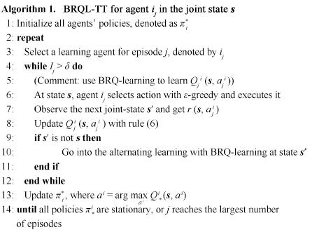
In the end,the multi-agent reinforcement learning BRQL-TT is depicted in Algorithm 1.
In order to test the performance of BRQL-TT,we set up the simulation of box-pushing[20]. Besides BRQL-TT,other two classical and recent algorithms are selected for comparison. One is WoLF-PHC,in which the learning principle is "learn quickly while losing,slowly while winning". The other is Hysteretic-Q, which is proposed to avoid the overestimation of Q-value. We run the experiment 50 times,and the agents learn till finishing the task with the above algorithms in the 300 000 steps every time.
A. Setup of ExperimentIn Fig. 2,a rectangular environment is assumed. Several fixed obstacles are distributed randomly in the environment. In addition,in order to alleviate programming burden,the object is simplified as a square box in the lower left corner. There are four agents (robots) around the square,denoted by circles in the environment. It is assumed that the box is sufficiently big and heavy so that any individual robot cannot handle it without the help of the peer robots. The agents and the box share the same state space,which is divided into grids of $10 \times 15$ for creating Q-tables. And the actions of agents include the force and its direction angle.

|
Download:
|
| Fig. 2. The box-pushing problem and the definition of action: force and direction. | |
The valid actions include force $\times$ direction. Scale of this space is ${\rm linspace}(0,1,5) \times {\rm linspace}(0,2\pi ,10)$. The parameters of RL are set as $\gamma = 0.95$, ${\alpha _t} = 1/(t + 1)^{0.018}$. We use the $\varepsilon$-greedy for decision making,and set $\varepsilon = 0.2$ initially which is decreased slowly. And the individual reward is $1$ when the agents push the box to the goal,otherwise,$-1$ as penalty. And the initial Q-value for all agents is $-50$. In addition to the basic parameters which is the same as BRQL-TT,the parameters of WoLF-PHC are ${\delta _{win}} = 0.03$,${\delta _{lose}}=0.06$,and those of Hysteretic-Q are $\alpha=0.3$,$\beta$ = 0.03[15].
B. Dynamic Process of BRQL-TTWe focus on one state. Fig. 3 shows the order of learning agents over the first 1000 times of visiting state [14, 8]. Initially, agent 3 (marked by cross),is assigned as the first learning agent. After nearly 400 steps,agent 3 obtains the best response to the others,and lets agent 2 (marked by star) take its place of learning according to the switching rule,then agent 4,agent 2, and agent 3 repeatedly. Finally,because EDR of [14, 8] almost converges,the switch of learning agents becomes more and more quickly.

|
Download:
|
| Fig. 3. The learning order of agents sampled from the state [14, 8]. | |
Since the state space of box-pushing problem is 2D,the V-values (maximum of Q-value over agents' actions) of all joint states with respect to four agents can be mapped to a 3D plot as shown in Fig. 4. Theorem 1 implies that,according to the definition of EDR,the cooperative learning with TTF will result in the same V-values map for all agents. Fig. 4 shows this property,where the goal of box-pushing is set to be the state [14, 9].

|
Download:
|
| Fig. 4. V-values over 2D-state space w.r.t. four agents. | |
To investigate this property in details,we map the 2D states into linear horizon axis according to the indices assigned to them,and depict all V-values with respect to the four agents in Fig. 5. Clearly,for the states close to the goal,which are indicated by relatively higher V-values,their V-values are more identical. It implies that the states around the goal are exploited more thoroughly than others.

|
Download:
|
| Fig. 5. V-values corresponding to the states indexed in linear axis. | |
In this subsection,some results and comparison between our algorithm BRQL-TT and other algorithms (WoLF-PHC and Hysteretic-Q) will be discussed. Figs. 6 and 7 show the average steps and average reward obtained by agents over 50 times of the experiment. Table 1 shows the detail learning results about memory cost and converged steps.

|
Download:
|
| Fig. 6. Average steps required to complete a trial. | |

|
Download:
|
| Fig. 7. Average reward obtained in every trial. | |
|
|
TABLE Ⅰ COMPARISON IN THE SPACE COST AND CONVERGED STEPS |
The curves marked by circles in Figs. 6 and 7 show the evolution of average steps and rewards with BRQL-TT as the learning steps increase till 300 000. The low average steps and the high average reward indicate efficiency of our algorithm. The curves marked by diamonds which results from Hysteretic-Q shows that it can hardly converge in the same number of steps,while the learning with WoLF-PHC,denoted by the curves marked by squares,shows the best converging ability. Thus roughly speaking,the proposed algorithm always outperforms Hysteretic-Q,and is close to WoLF-PHC in converging ability. More properties of dynamics are summarized as follows.
Firstly,Figs. 6 and 7 show the learning performance from the beginning to the end. Due to the fewer steps needed in one trail, BRQL-TT learns with less exploration cost than the other two algorithms in the first half period of the experiment. Although the learning using WoLF-PHC is more effective than BRQL-TT after 200 000 steps,BRQL-TT looks more steady in the whole learning process. These comparisons tell that,if we take the learning algorithms into applications that cannot afford the high price of exploration,BRQL-TT is a good choice among the three.
Secondly,although TTF makes agents learn in a serial way,but not in a parallel way,the alternate learning does not prolong the learning process significantly. And such alternate learning drives MAS to maintain strong exploration behavior for a long period. That may be the reason for better performance.
Finally,it is easy to investigate that the space cost of the proposed algorithm is $N \cdot \left| S \right| \cdot |A|$,which is the same as Hysteretic-Q. However,the space required by WoLF-PHC is doubled,since the agents must build the table for their strategies such as Q-value. All data is shown in Table Ⅰ. On the other hand, as only one agent learns in each state when using BRQL-TT,the computational cost will be much less than those of the other two algorithms.
Above all,the simulation results show feasibility of TTF and high efficiency of BRQL-TT in cooperative reinforcement learning. In addition,in the aspects of applicable conditions,exploration cost,reproducibility of dynamics,BRQL-TT shows its special characteristics and superiorities.
Ⅴ. CONCLUSIONS AND FUTURE WORKTo tackle cooperative multi-agent learning without knowledge about companions' policies in priori,this paper firstly gives two assumptions to analyze what is brought by individual learning to group policy. Based on the common EIR,EDR is proposed to measure effectiveness of cooperation under the pure policies taken by agents. Then,TTF is proposed to make individual agents have chances to develop EDR in every joint state. To decrease the dimension of action and enhance efficiency of individual learning, BRQ-learning is developed to entitle agents to get the best responses to their companions,or in other words,track its companion's behavior. Finally,with BRQL-TT applied with TTF,the EDR under the cooperative policy of MAS increases consistently and converges finally. Due to significant decrease in the dimension of action space,the algorithm speeds up the learning process,and reduces computation complexity. It is attractive for the implementation of cooperative MAS.
EDR defined in this paper can be viewed as a general expression about the discounted reward of MAS,so that the discounted reward based on joint-state joint-action will be regarded as a special EDR resulting from all agents executing the pure policies. Thus, the cooperative learning is transformed into a kind of EDR optimization,which consists of individual learning and coordinate optimization of EDR. So the convergence theorem on the simultaneous learning in the decentralized way will be our main work in the future.
| [1] | Gao Yang, Chen Shi-Fu, Lu Xin. Research on reinforcement learning technology:a review. Acta Automatica Sinica, 2004, 30(1):86-100(in Chinese) |
| [2] | Busoniu L, Babuska R, Schutter B D. Decentralized reinforcement learning control of a robotic manipulator. In:Proceedings of the 9th International Conference on Control, Automation, Robotics and Vision. Singapore, Singapore:IEEE, 2006. 1347-1352 |
| [3] | Maravall D, De Lope J, Douminguez R. Coordination of communication in robot teams by reinforcement learning. Robotics and Autonomous Systems, 2013, 61(7):661-666 |
| [4] | Gabel T, Riedmiller M. The cooperative driver:multi-agent learning for preventing traffic jams. International Journal of Traffic and Transportation Engineering, 2013, 1(4):67-76 |
| [5] | Tumer K, Agogino A K. Distributed agent-based air traffic flow management. In:Proceedings of the 6th International Joint Conference on Autonomous Agents and Multiagent Systems. Honolulu, Hawaii, USA:ACM, 2007. 330-337 |
| [6] | Tang Hao, Wan Hai-Feng, Han Jiang-Hong, Zhou Lei. Coordinated lookahead control of multiple CSPS system by multi-agent reinforcement learning. Acta Automatica Sinica, 2010, 36(2):330-337(in Chinese) |
| [7] | Busoniu L, Babuska R, De Schutter B. A comprehensive survey of multiagent reinforcement learning. IEEE Transactions on Systems, Man, and Cybernetics-Part C:Applications and Reviews, 2008, 38(2):156-172 |
| [8] | Abdallah S, Lesser V. A multiagent reinforcement learning algorithm with non-linear dynamics. Journal of Artificial Intelligence Research, 2008, 33:521-549 |
| [9] | Xu Xin, Shen Dong, Gao Yan-Qing, Wang Kai. Learning control of dynamical systems based on Markov decision processes:research frontiers and outlooks. Acta Automatica Sinica, 2012, 38(5):673-687(in Chinese) |
| [10] | Fulda N, Ventura D. Predicting and preventing coordination problems in cooperative Q-learning systems. In:Proceedings of the 20th International Joint Conference on Artificial Intelligence. San Francisco, CA, USA:Morgan Kaufmann Publishers Inc, 2007. 780-785 |
| [11] | Chen X, Chen G, Cao W H, Wu M. Cooperative learning with joint state value approximation for multi-agent systems. Journal of Control Theory and Applications, 2013, 11(2):149-155 |
| [12] | Wang Y, de Silva C W. Multi-robot box-pushing:single-agent Qlearning vs. team Q-learning. In:Proceedings of IEEE/RSJ International Conference on Intelligent Robots and Systems. Beijing, China:IEEE, 2006. 3694-3699 |
| [13] | Cheng Yu-Hu, Feng Huan-Ting, Wang Xue-Song. Expectationmaximization policy search with parameter-based exploration. Acta Automatica Sinica, 2012, 38(1):38-45(in Chinese) |
| [14] | Teboul O, Kokkinos I, Simon L, Koutsourakis P, Paragios N. Parsing facades with shape grammars and reinforcement learning. IEEE Transactions on Pattern Analysis and Machine Intelligence, 2013, 35(7):1744-1756 |
| [15] | Matignon L, Laurent G J, Fort-Piat N L. Independent reinforcement learners in cooperative Markov games:a survey regarding coordination problems. The Knowledge Engineering Review, 2012, 27:1-31 |
| [16] | Bowling M, Veloso M. Multiagent learning using a variable learning rate. Artificial Intelligence, 2002, 136(2):215-250 |
| [17] | Kapetanakis S, Kudenko D. Reinforcement learning of coordination in heterogeneous cooperative multi-agent systems. In:Proceedings of the Third International Joint Conference an Autonomous Agents and Multiagent System. New York, USA:IEEE, 2004. 1258-1259 |
| [18] | Matignon L, Laurent G J, Fort-Piat N L. Hysteretic Q-learning:an algorithm for decentralized reinforcement learning in cooperative multiagent teams. In:Proceedings of IEEE/RSJ International Conference on Intelligent Robots and System. San Diego, California, USA:IEEE, 2007. 64-69 |
| [19] | Tsitsiklis J N. On the convergence of optimistic policy iteration. The Journal of Machine Learning Research, 2003, 3:59-72 |
| [20] | Wang Y, de Silva C W. A machine-learning approach to multi-robot coordination. Engineering Applications of Artificial Intelligence, 2008, 21(3):470-484 |