 2014, Vol.1


2. Key Laboratory of Intelligent Control and Decision of Complex Systems, Beijing Institute of Technology, Beijing 100081, China;
3. School of Automation, Beijing Institute of Technology, Beijing 100081, China;
4. School of Automation, Beijing Institute of Technology, Beijing 100081, China;
5. School of Computing and Mathematics, Plymouth University, Plymouth PL4 8AA, UK;
6. School of Automation, Beijing Institute of Technology, Beijing 100081, China
T he concept of multi-agent systems[1, 2, 3, 4, 5, 6, 7] is proposed in 1980s with the development of complex system theory. Through the approach of dividing and conquering,decomposing a large complex system into small components or subsystems,which have intrinsic local coupling relations with each other,is a promising idea which can greatly simplify the control design of the whole system and reduce the total computational cost significantly. Hence understanding how local interactions affect the global behavior plays fundamental role either in theory or in practice.
A multi-agent system,as one simplified model for investigating complex systems,is composed of many agents which not only have local interactions among one another but also respond to others by making decisions and taking actions. In this way,the agents can perform one simple task independently or complete one difficult task by cooperation and communication. Based on the above features,many applications of multi-agent systems can be found in vast areas,such as intelligent robot[8, 9],smart home system[10], aerospace field[11],intelligent transportation system (ITS)[12, 13],software development and so on.
There are many kinds of research about multi-agent systems in recent years. Main research topics may include the architecture of the multi-agent system,the communication among agents,coordination and cooperation. The architecture discusses how the agents form the system and the communication discusses the way in which information transfers among agents. The coordination control of the multi-agent system is comprehensive,since this problem needs to consider the architecture and communication. And consensus control of multiple agents as one kind of coordination control has received more and more attentions in the recent decades. Consensus means the agents can make their states and velocities in agreement by cooperation and communication. This problem was first proposed by Olfati-Saber and Murray[14]. In the direction of distributed consensus in multi-agent cooperative control,Ren et al. have obtained numerous results[15, 16, 17]. These existing extensive work presented the consensus algorithms for single-integrator dynamics, double-integrator dynamics and rigid body attitude dynamics.
However,many studies about multi-agent systems assume that the global team knowledge is available,that is,the relations among agents are known,and the group actions can be achieved in a centralized way. The situations where there are unknown or uncertain relations between agents are basically ignored for decades. %in a long time. In fact,these situations have important effects on the studies of multi-agent systems which often exist in the practical applications. In such situations,the agents must try to cope with the uncertainties occurred in local interactions with only limited available history information and local information.
In this paper,we try to elaborate the decentralized filtering problem of one typical class of multi-agent systems,which focuses on dealing with coupling uncertainties. In such systems,there are unknown couplings among agents. As a preliminary study,in this paper we use linear mappings to represent such unknown interactions briefly. Due to the unknown couplings among agents,common filter algorithms like standard Kalman filters[18, 19, 20, 21, 22, 23, 24] cannot be used directly. To address this challenging problem,in this contribution, the filtering process is achieved by adopting modifications to standard Kalman filter algorithm. This area is less explored in the existing literature despite that another challenging area, decentralized adaptive control of multi-agent systems,has been extensively studied by the authors[25],hence this paper aims to lay a simple yet meaningful framework of decentralized adaptive filtering for multi-agent systems. Because of intrinsic differences between linear systems and nonlinear systems,we classify the considered system models as four different types according to the model linearity and the coupling type,and hence different decentralized filtering algorithms should be designed separately. And through estimated values of the states obtained by decentralized adaptive filtering,corresponding decentralized adaptive control law is designed according to the certainty equivalence principle. The stability of the filtering algorithm is also discussed with verification by simulations.
The rest of this paper is organized as follows. First,Section II presents the system model and problem formulation. Then,in Section III,the decentralized adaptive filtering algorithms are derived. Next in Section IV,based on the certainty equivalence principle, decentralized adaptive controller is designed to test the filtering effects. In Section V,some remarks on the stability analysis for the proposed decentralized filtering algorithms are given. And,in Section VI,simulations of decentralized adaptive filter and control algorithms are reported and the corresponding results are analyzed. Finally,we conclude this paper with some concluding remarks in Section VII.
Notations 1. The following notations are used throughout this paper. ${\bf R}^n$ and ${\bf R}^{m}$ stand for the set of real vectors with dimension $n$ and $m$ respectively. $I$ and $0_{m\times n}$ mean the identity matrix and zero matrix. The subscript of matrix represents the dimension of the matrix of dimension $m$ by $n$. Wherever the dimensions of the matrices are not mentioned,they are assumed to be of compatible dimensions. E($\cdot$) and $P(\cdot)$ denote the mathematical expectation and variance. ${\left[ \cdot \right]^T}$ denotes the transposition of a matrix and $(\cdot)^{-1}$ denotes the inversion of a matrix. $\widehat *$ and $\bar *$ on the top represent the corresponding posterior and prior terms,respectively.
II. PROBLEM STATEMENTSince agents often have similar structures and the same state dimension,we assume $x_{i}\in {\bf R}^{n}$,$u_{i}\in {\bf R}^{r}$, $y_{i}\in {\bf R}^{m}$,$w_{i}$ $\in$ ${\bf R}^{n}$ and $v_{i}\in {\bf R}^{m}$ for every $i$ in $\{1,2,\cdots,N\}$.
A.Model 1: Linear Model with Output Coupling
Considering one class of multi-agent system where there are $N$
agents and every agent can be described by the following dynamic
model:
\begin{align}
x_{i}(k)=&\ A_{i}(k-1)x_{i}(k-1)+B_{i}(k-1)u_{i}(k-1) +\nonumber \\
&\sum_{j_{p}\in\Bbb N_{i}}q_{i,j_p} G_{i,j_{p}}y_{j_{p}}(k-1)+w_{i}(k-1), \nonumber \\
y_{i}(k)=&\ C_{i}(k)x_{i}(k)+v_{i}(k), \nonumber \\
\Bbb N_{i}=&\ \{j_{1},j_{2},\cdots,j_{n_{i}}\},
\end{align}
(1)
\begin{align}
x_{i}(k)
=&\ A_{i}(k-1)x_{i}(k-1)+B_{i}(k-1)u_{i}(k-1) + \nonumber \\
& \sum_{j_{p}\in\Bbb N_{i}}q_{i,j_{p}} y_{j_{p}}(k-1)+w_{i}(k-1).
\end{align}
(2)
\begin{align}
x_{i}(k)
=\ A_{i}(k-1)x_{i}(k-1)+B_{i}(k-1)u_{i}(k-1) + \\
\sum_{j_{p}\in\Bbb N_{i}}q_{i,j_{p}}x_{j_{p}}(k-1)+w_{i}(k-1), \\
y_{i}(k) =\ C_{i}(k)x_{i}(k)
+v_{i}(k), \\
\Bbb N_{i}=\ \{j_{1},j_{2},\cdots,j_{n_{i}}\},\label{eq.model2}
\end{align}
(3)
Each agent $i$ has the following nonlinear dynamics
\begin{align}
x_{i}(k)
=&\ f_{i}(x_{i}(k-1),w_{i}(k-1))+B_{i}(k-1) \times \\
&\ u_{i}(k-1)+\sum_{j_{p}\in\Bbb N_{i}}q_{i,j_{p}}g_{i,j_{p}}(y_{j_{p}}(k-1)), \\
y_{i}(k)
=&\ h_{i}(x_{i}(k),v_{i}(k)) , \\
\Bbb N_{i}=&\ \{j_{1},j_{2},\cdots,j_{n_{i}}\},\label{eq.model3}
\end{align}
(4)
D.Model 4: Nonlinear Model with State Coupling
The dynamic model of every agent is
\begin{align}
x_{i}(k)
=&\ f_{i}(x_{i}(k-1),w_{i}(k-1))+B_{i}(k-1) \times \\
&\ u_{i}(k-1)+\sum_{j_{p}\in\Bbb N_{i}}q_{i,j_{p}}g_{i,j_{p}}(x_{j_{p}}(k-1)), \\
y_{i}(k)
=&\ h_{i}(x_{i}(k),v_{i}(k)), \\
\Bbb N_{i}=&\ \{j_{1},j_{2},\cdots,j_{n_{i}}\},\label{eq.model4}
\end{align}
(5)
In the four models,the subscripts $i$ and $j_{p}$ denote the $i${th} and $j_{p}${th} agent. Here $x_{i}(k)$ and $x_{i}(k-1)$ are the states of $i${th} agent in the $k${th} and $(k-1)${th} moment,respectively. Accordingly $x_{j_{p}}(k-1)$ denotes the state of $j_{p}${th} agent in the $(k-1)${th} moment. And $y$,$u$,$w$,and $v$ denote the output,input,process noise,and measurement noise,respectively. The inputs are written as the above since they are designed to test effects of the estimation. The difference is that agents are linear in Model 1 and Model 2,but agents are nonlinear in Model 3 and Model 4. And agents in Model 1 and Model 3 are coupled by outputs and in Model 2 and Model 4 they are coupled by states.
The coupling term $\sum_{j_{p}\in\Bbb N_{i}}q_{i,j_{p}}g_{i,j_{p}}(x_{j_{p}}(k-1))$ shows influence between agents and their neighbor agents,where scalar $q_{i,j_p}$ denotes the corresponding coupling strength. To simplify the unknown relations,we use unknown parameters $q_{i,j_p}$ and known functions $g_{i,j_{p}}(k-1)$ to present the coupling structure. And this term represents the influence of neighbor agent $j_{p}$ on agent $i$. The index set $\Bbb N_{i}$ denotes the set of agents which have effects on agent $i$.
Suppose that the noises are white,zero-mean,uncorrelated and the
noises of different agents are also uncorrelated. If the noises are
correlated,we can also use methods proposed in the book written by
Simon[19] to remove the correlation.
% There are also some explanations about noises that need to be shown:
For simplicity and clarity,we may suppose that the {a priori}
statistical information on noises are given by
\begin{align}
w_{i}(k)\sim&\ {\rm N}(0,Q_{i}(k)), \\
v_{i}(k)\sim&\ {\rm N}(0,R_{i}(k)).
\end{align}
(6)
The whole description of the multi-agent dynamic system is shown above. Among the four models,Model 1 and Model 2 are basis of Model 3 and Model 4,hence the understanding of the former two models will bring benefits to the latter two models. However,due to the nonlinearity of Model 3 and Model 4,they are more challenging in terms of closed-loop complexity and technical difficulties involved, and later we may see that different algorithms may be needed in general for resolving the decentralized adaptive filtering problems for different models. For achieving control objectives of agents,it would be desirable that the states need to be known. Since the system has unknown parameters,we cannot estimate the states only by standard Kalman filter,hence new filter algorithm needs to be studied to estimate the states and coupling parameters in the linear state-space model.
III.DECENTRALIZED ADAPTIVE FILTER
Firstly,the inputs are assumed to be zero for they are only testing
terms and cannot affect the study of filter algorithm. And the first
step to deal with the unknown coupling parameters $q_{i,j_{p}}$ is
to consider the coupling parameters as a part of states,that is,to
extend the states. The new state vector is changed to
\begin{equation}
%\label{eq1}
x_{i}^{*}(k)= \left[\begin{array}{c}
x_{i}(k)\\
q_{i,j_{1}}\\
q_{i,j_{2}}\\
\vdots\\
q_{i,j_{n_{i}}}\\
\end{array}\right]_{(n+n_{i})\times 1}.
\end{equation}
(7)
A.Model 1
The algorithm is based on the standard Kalman filter and a
decentralized one. With the augmented states,the dynamic model of
original multi-agent system can be rewritten as follows:
\begin{align}
x_{i}^{*}(k)
=&\ A_{i}^{*}(k-1)x_{i}^{*}(k-1)+w_{i}^{*}(k-1), \\
y_{i}^{*}(k)=&\ y_{i}(k)= % \\ &
C_{i}^{*}(k)x_{i}^{*}(k)+v_{i}^{*}(k) ,\label{eq.model1.new}
\end{align}
(8)
\begin{align}
A_{i}^{*}(k-1) \!=\!
\left[\begin{array}{ccccc}
A_{i}(k-1)&G_{i,j_{1}} y_{j_{1}}(k-1)&\cdots&G_{i,j_{n_{i}}} y_{j_{n_{i}}}(k-1) \\
0_{1\times n}&1&\cdots&0 \\
0_{1\times n}&0&\cdots&0 \\
\vdots&\vdots&\ddots&\vdots\\
0_{1\times n}&0&\cdots&1 \\
\end{array}\right],
\label{eq.Ai.11}
\end{align}
(9)
\begin{align}
&C^{*}_{i}(k)= \left[
%\begin{array}{c}
C_{i}(k),%
0_{m\times 1},%
0_{m\times 1},%
\cdots,%
0_{m\times 1}%
%\end{array}
\right]_{m\times (n+n_{i})} , \\
&w_{i}^{*}(k-1) =\left[\begin{array}{c}
I_{n\times n}\\
0_{1\times n}\\
0_{1\times n}\\
\vdots\\
0_{1\times n}\\
\end{array}\right]_{(n+n_{i}) \times n}\times w_{i}(k-1), \\
&v_{i}^{*}(k) =v_{i}(k),
\end{align}
(10)
\begin{align}
w_{i}^{*}(k) \sim&\ {\rm N}(0,Q_{i}^{*}(k)),\\
v_{i}^{*}(k)
\sim&\ {\rm N}(0,R_{i}^{*}(k)) , \\
Q_{i}^{*}(k) =&\ \left[\begin{array}{cc}
Q_{i}(k)&0_{n\times n_{i}}\\
0_{n_{i}\times n}&0_{n_{i}\times n_{i}}\\
\end{array}\right]_{(n+n_{i})\times (n+n_{i})} ,\end{align}
\begin{align}
R_{i}^{*}(k) =&\ R_{i}(k).
\end{align}
(11)
\begin{align}
\bar P_{i}^{*}(k)
=&\ A_{i}^{*}(k-1)\widehat P_{i}^{*}(k-1)[{A_{i}^{*}(k-1)}]^{\rm T}+Q_{i}^{*}(k-1), \\
K_{i}^{*}(k)
=&\ \bar P_{i}^{*}(k)[{C_{i}^{*}(k)}]^{\rm T} \{C_{i}^{*}(k)\bar P_{i}^{*}(k)[{C_{i}^{*}(k)}]^{\rm T}\!+\!% \\
%&
R_{i}^{*}(k)\}^{-1} , \\
\bar x_{i}^{*}(k)
=&\ A_{i}^{*}(k-1)\widehat x_{i}^{*}(k-1) , \\
\widehat x_{i}^{*}(k)
=&\ \bar x_{i}^{*}(k)+K_{i}^{*}(k)(y_{i}^{*}(k)-C_{i}^{*}(k)\bar x_{i}^{*}(k)), \\
\widehat P_{i}^{*}(k)
=&\ [I-K_{i}^{*}(k)C_{i}^{*}(k)]\bar P_{i}^{*}(k)[{I-K_{i}^{*}(k)C_{i}^{*}(k)}]^{\rm T} + \\
&\ K_{i}^{*}(k)R_{i}^{*}(k)K_{i}^{*}(k),
\end{align}
(12)
${\bf Algorithm 1.}$ ${\bf Decentralized filter for linear system (DFL)}$
${\bf Input.}$ Coefficient matrices,neighborhood indices and outputs of every agent.
${\bf Output.}$ Estimated values of states and coupled parameters.
1 Extend dimensions of states;
2 Update the state equations using the new extending states;
3 Initialize estimation values and calculate the initial error covariance matrix;
4 Initialize simulation steps $T$;
5 ${\bf for}$ $k=2$ to $T$ ${\bf do}$
6 ${\bf for}$ $i=1$ to $N$ ${\bf do}$
7 Form matrix $A_{i}^{*}(k)$ with neighbor outputs $y_{j_{l}}$ via (9);
8 Calculate the next prior error covariance $\bar P_{i}^{*}(k)$ via (12);
9 Calculate the Kalman gain matrix $K^{*}_{i}(k)$ via (12);
10 Time update --- calculate $\bar x_{i}^{*}(k)$ from $\widehat x_{i}^{*}(k-1)$ via (12);
11 Measurement update --- calculate $\widehat x_{i}^{*}(k)$ with $K_{i}^{*}(k)$via (12) as new measurement $y_{i}^{*}(k)$ is available;
12 Calculate the posterior error covariance $\widehat P_{i}^{*}(k)$ via (12);
13 ${\bf end for}$
14 ${\bf end for}$
15 Output and display sequences of $\widehat x_{i}^{*}(k)$ which contains estimation of coupled parameters and states;
16 ${\bf end}$}
B.Model 2
This algorithm is based on the standard Kalman filter and a
decentralized one. With the augmented states,the dynamic model of
original multi-agent system can be rewritten as follows:
\begin{align}
x_{i}^{*}(k)
=&\ A_{i}^{*}(k-1)x_{i}^{*}(k-1)+w_{i}^{*}(k-1), \\
y_{i}^{*}(k)=&\ y_{i}(k)= % \\
%&
C_{i}^{*}(k)x_{i}^{*}(k)+v_{i}^{*}(k),\label{eq.model2.new}
\end{align}
(13)
\begin{equation}
A_{i}^{*}(k-1)
=\left[\begin{array}{ccccc}
A_{i}(k-1)&x_{j_{1}}(k-1)&x_{j_{2}}(k-1)&\cdots&x_{j_{n_{i}}}(k-1) \\
0_{1\times n}&1&0&\cdots&0 \\
0_{1\times n}&0&1&\cdots&0 \\
\vdots&\vdots&\vdots&\ddots&\vdots\\
0_{1\times n}&0&0&\cdots&1 \\
\end{array}\right].
\end{equation}
(14)
Except for matrix $A_{i}^{*}(k-1)$,other terms are the same with
Model $1$. The new problem is that some terms of $A_{i}^{*}(k-1)$
are unknown,hence the standard Kalman filter cannot be applied to
the modified model directly. Since agents can communicate with each
other,the estimated values of these unknown ones can be transmitted
to replace the real values. That is,in the filtering process of
Model $1$,the matrix $A_{i}^{*}(k-1)$ is changed to
\begin{equation}
A_{i}^{*}(k-1)
=\left[\begin{array}{ccccc}
A_{i}(k-1)&\widehat x_{j_{1}}(k-1)&\widehat x_{j_{2}}(k-1)&\cdots&\widehat x_{j_{n_{i}}}(k-1) \\
0_{1\times n}&1&0&\cdots&0 \\
0_{1\times n}&0&1&\cdots&0 \\
\vdots&\vdots&\vdots&\ddots&\vdots\\
0_{1\times n}&0&0&\cdots&1 \\
\end{array}\right] ,\label{eq.Ai.2}
\end{equation}
(15)
${\bf Algorithm 2.}$ ${\bf Decentralized filter for linear system 2 (DFL2)}$
${\bf Input.}$ Coefficient matrices,neighborhood indices and outputs of every agent.
${\bf Output.}$ Estimated values of states and coupled parameters.
1 Extend dimensions of states;
2 Update the state equations using the new extending states;
3 Initialize estimation values and calculate the initial error covariance matrix; 4 Initialize simulation steps $T$;
5 ${\bf for}$ $k=2$ to $T$ ${\bf do}$
6 ${\bf for}$ $i=1$ to $N$ ${\bf do}$
7 Form matrix $A_{i}^{*}(k)$ via (15) with neighbor outputs $\widehat x_{j_{p}}$ ($j_{p}\in\Bbb N_{i}$);
8 Calculate the next prior error covariance $\bar P_{i}^{*}(k)$ via (12);
9 Calculate the Kalman gain matrix $K^{*}_{i}(k)$ via (12);
10 Time update --- calculate $\bar x_{i}^{*}(k)$ from $\widehat x_{i}^{*}(k-1)$ via (12);
11 Measurement update --- calculate $\widehat x_{i}^{*}(k)$ with $K_{i}^{*}(k)$ via(12) as new measurement $y_{i}^{*}(k)$ is available; 12 Get the posterior error covariance matrix $\widehat P_{i}^{*}(k)$ via (12);
13 ${\bf end for}$
14 ${\bf end for}$
15 Output and display sequences of $\widehat x_{i}^{*}(k)$ which contains estimation of coupled parameters and states;
16 ${\bf end}$}
C.Model 3
Since the model is nonlinear,the extended Kalman filter can be
considered as the basic algorithm. Firstly,using the same notations
$x_{i}^{*}(k)$,$w_{i}^{*}(k)$,$v_{i}^{*}(k)$ as in Model 1,we
obtain the modified model of agent dynamics
\begin{align}
x_{i}^{*}(k)
=&\ f_{i}^{*}(x_{i}^{*}(k),w_{i}^{*}(k-1)),\\
y_{i}^{*}(k)=&\ y_{i}(k) = % \\
%&
h_{i}^{*}(x_{i}^{*}(k),v_{i}^{*}(k-1)) ,\label{eq.model3.new}
\end{align}
(16)
\begin{align}%
&x_{i}^{*}(k)=\left[\begin{array}{c}
f_{i}(\cdots)+\sum\limits_{j_{p}\in\Bbb N_{i}}q_{i,j_{p}}g_{i,j_{p}}(y_{j_{p}}(k-1))\\
q_{i,j_{1}}\\
q_{i,j_{2}}\\
\vdots\\
q_{i,j_{n_{i}}}
\end{array}\right],\end{align}
(17)
\begin{align}%
& y_{i}^{*}(k)=y_{i}(k)=h_{i}(x_{i}(k),v_{i}(k)).
\end{align}
(18)
Then we find that the problem of simultaneously estimating the unknown states and the coupling parameters can be transformed to a filter problem of the new model,i.e. estimating the augmented states $x_{i}^{*}(k)$. The new model is a nonlinear dynamic model, hence the extended Kalman filter algorithm[26] can be applied in this modified model. For clarity,the filtering process is shown as follows.
${\bf The filtering process.}$
1) Calculate partial derivatives matrices of
functions
\begin{align}%
A_{i}^{*}(k-1)=&\ \frac{\partial f_{i}^{*}}{\partial
x_{i}^{*}}|_{\widehat x_{i}^{*}(k-1)},\label{eq.Ai.3}
\end{align}\begin{align}\end{align}
(19)
\begin{align}%
G_{i}^{*}(k-1)=&\ \frac{\partial f_{i}^{*}}{\partial
w_{i}}|_{\widehat x_{i}^{*}(k-1)},\label{eq.Gi.3}
\end{align}
(20)
2) Time update
\begin{align}%
\bar P_{i}^{*}(k)=&\ A_{i}^{*}(k-1)\widehat P_{i}^{*}(k-1)[{A_{i}^{*}(k-1)}]^{\rm T} + \\
&\ G_{i}^{*}(k-1)Q_{k-1}[{G_{i}^{*}(k-1)}]^{\rm T}, \\
\bar x_{i}^{*}(k)=&\ f_{i}^{*}(\widehat x_{i}^{*}(k-1),0_{n\times
n}).
\end{align}
(21)
3) Calculate partial derivatives matrices of functions
\begin{align}%
C_{i}^{*}(k)=&\ \frac{\partial h_{i}^{*}}{\partial x_{i}^{*}}|_{\bar
x_{i}^{*}(k)},\label{eq.Ci.3}
\end{align}
(22)
\begin{align}%
J_{i}^{*}(k)=&\ \frac{\partial h_{i}^{*}}{\partial v_{i}}|_{\bar
x_{i}^{*}(k)},\label{eq.Ji.3}
\end{align}
(23)
4) Measurement update
\begin{align}%
K_{i}^{*}(k)=&\ \bar P_{i}^{*}(k)[{C_{i}^{*}(k)}]^{\rm
T}\{C_{i}^{*}(k)\bar P_{i}^{*}(k)[{C_{i}^{*}(k)}]^{\rm
T}+R_{k}\}^{-1},\label{eq.Ki.3}
\\
\widehat x_{i}^{*}(k)=&\ \bar
x_{i}^{*}(k)+K_{i}^{*}(k)[y_{i}^{*}(k)-h_{i}^{*}(\bar
x_{i}^{*}(k),0_{m\times m})],
\\
\widehat P_{i}^{*}(k)=&\ [I-K_{i}^{*}(k)C_{i}^{*}(k)]\bar
P_{i}^{*}(k).
\end{align}
(24)
${\bf Input.}$ Functions,neighborhood indices and outputs of every agent.
${\bf Output.}$ Estimated values of states and coupled parameters.
1 Extend dimension of states;
2 Update the state equations using the new extending states;
3 Initialize estimation values and calculate the initial error covariance matrix;
4 Initialize simulation steps $T$;
5 ${\bf for}$ $k=2$ to $T$ ${\bf do}$
6 ${\bf for}$ $i=1$ to $N$ ${\bf do}$
7 Form $A_{i}^{*}(k)$ and $G_{i}^{*}(k-1)$ via (19) and (20) with $\widehat x_{i}^{*}(k-1)$ and $y_{j_{p}}$ ($j_{p}\in\Bbb N_{i}$);
8 Calculate the next prior error covariance $\bar P_{i}^{*}(k)$ via (21);
9 Time update --- calculate $\bar x_{i}^{*}(k)$ from $\widehat x_{i}^{*}(k-1)$ via (21);
10 Calculate matrices $C_{i}^{*}(k)$ and $J_{i}^{*}(k)$ via (22) and (23);
11 Calculate the Kalman gain matrix $K_{i}^{*}(k)$ via (24);
12 Measurement update --- calculate $\widehat x_{i}^{*}(k)$ with $K_{i}^{*}(k)$ via (24) as new measurement $y_{i}^{*}(k)$ is available;
13 Get the posterior error covariance matrix $\widehat P_{i}^{*}(k)$ via (24);
14 ${\bf end for}$
15 ${\bf end for}$
16 Output and display sequences of $\widehat x_{i}^{*}(k)$ which contains estimation of coupled parameters and states;
17 ${\bf end}$}
D.Model 4
Rewriting the dynamic model,we can obtain a similar model as given
above. The difference is the state equation as follows:
\begin{equation}%
x_{i}^{*}(k)=\left[\begin{array}{c}
f_{i}(\cdot)+\sum\limits_{j_{p}\in\Bbb N_{i}}q_{i,j_{p}}g_{i,j_{p}}(x_{j_{p}}(k-1))\\
q_{i,j_{1}}\\
q_{i,j_{2}}\\
\vdots\\
q_{i,j_{n_{i}}}
\end{array}\right].
\end{equation}
(25)
There are terms which are different from output coupling of Model
$3$,such as $g_{i,j_{1}}(x_{j_{1}}(k-1))$. That is,when partial
derivatives matrices of functions are calculated,these terms are
unknown which are different from terms only including outputs.
Hence,some modifications are necessary to extend the algorithm.
Since posterior estimation values are close to the true values,we
use the posterior estimation instead.
\begin{align}%
A_{i}^{*}(k-1)=&\ \frac{\partial f_{i}^{*}}{\partial
x_{i}^{*}}|_{\widehat x_{i}^{*}(k-1)},\label{eq.Ai.4}
\end{align}
(26)
\begin{align}%
G_{i}^{*}(k-1)=&\ \frac{\partial f_{i}^{*}}{\partial
w_{i}}|_{\widehat x_{i}^{*}(k-1)}.\label{eq.Gi.4}
\end{align}
(27)
${\bf Algorithm 4.}$ ${\bf Decentralized filter for nonlinear system 2 (DFNL2)}$
${\bf Input.}$ Functions,neighborhood indices and outputs of every agent.
${\bf Output.}$ Estimated values of states and coupled parameters.
1 Extend dimensions of states;
2 Update the state equations using the new extending states;
3 Initialize estimation values and calculate the initial error covariance matrix;
4 Initialize simulation steps $T$;
5 ${\bf for}$ $k=2$ to $T$ ${\bf do}$
6 ${\bf for}$ $i=1$ to $N$ ${\bf do}$
7 Form $A_{i}^{*}(k)$ and $G_{i}^{*}(k-1)$ via (26) and (27) with $\widehat x_{i}^{*}(k-1)$;
8 Calculate the next prior error covariance $\bar P_{i}^{*}(k)$ via (21);
9 Time update --- calculate $\bar x_{i}^{*}(k)$ from $\widehat x_{i}^{*}(k-1)$ via (21);
10 Calculate matrices $C_{i}^{*}(k)$ and $J_{i}^{*}(k)$ via (22) and (23);
11 Calculate the Kalman gain matrix $K_{i}^{*}(k)$ via (24);
12 Measurement update --- calculate $\widehat x_{i}^{*}(k)$ with $K_{i}^{*}(k)$ via (24) as new measurement $y_{i}^{*}(k)$ is available;
13 Get the posterior error covariance matrix $\widehat P_{i}^{*}(k)$ via (24);
14 ${\bf end for}$
15 ${\bf end for}$
16 Output and display sequences of $\widehat x_{i}^{*}(k)$ which contains estimation of coupled parameters and states;
17 ${\bf end}$}
IV.DECENTRALIZED CONTROLLER DESIGNController design will be easy if the coupling parameters are exactly known {a priori}. However,since the coupling parameters are unknown in our settings,corresponding control parameters cannot be decided for the purpose of compensating the unknown coupling effects. To resolve this problem,one natural way is to regard the estimation of those parameters instead as their true values. This idea is in fact the so-called certainty equivalence principle,which is widely used in adaptive controller design. One can imagine that controllers based on this principle may yield satisfactory control performance if the parameter estimates are very close to the true parameters.
For testing estimation effects of filter algorithms,decentralized adaptive regulators are designed hereinafter. That is,control inputs are designed to regulate the states to zero based on the parameter estimates. For simplicity and clarity,coefficient matrices of inputs are assumed to be identity matrices,that is, $B_{i}(k-1)$ is equal to $I$.
For Model $1$,the control input of agent $i$\ can be designed as
follows:
\begin{equation}
u_{i}(k-1) =-A_{i}(k-1)\widehat
x_{i}(k-1)-\sum_{j_{p}\in\Bbb N_{i}}\widehat q_{i,j_{p}}y_{j_{p}}(k-1),
\end{equation}
(28)
For Model $2$,we have
\begin{equation}
u_{i}(k-1) =-A_{i}(k-1)\widehat
x_{i}(k-1)-\sum_{j_{p}\in\Bbb N_{i}}\widehat q_{i,j_{p}}\widehat
x_{j_{p}}(k-1).
\end{equation}
(29)
\begin{align}
u_{i}(k-1) =& -f_{i}(\widehat x_{i}(k-1),0_{n\times 1}) -
\notag\\
& \sum_{j_{p}\in\Bbb N_{i}}\widehat
q_{i,j_{p}}g_{i,j_{p}}(y_{j_{p}}(k-1)),
\end{align}
(30)
For Model $4$,we have
\begin{align}
u_{i}(k-1) =& -f_{i}(\widehat x_{i}(k-1),0_{n\times 1}) -\notag\\
& \sum_{j_{p}\in\Bbb N_{i}}\widehat q_{i,j_{p}}g_{i,j_{p}}(\widehat
x_{j_{p}}(k-1)).
\end{align}
(31)
If the estimation results are good enough,then control inputs designed as above can regulate states to zero approximately. In this way,the closed-loop signals may not diverge,consequently,the estimation results of filtering algorithms introduced before can be tested via simulations.
V.REMARKS ON STABILITY ANALYSIS
A.Linear Situations
The filtering process applied in the new Model $1$ is essentially
the standard Kalman filter for the augmented system. Though there
are some unknown coupling parameters,the new system obtained by
augmenting states can be considered as a normal multi-agent system
(8) without uncertain couplings. In the new augmented system model,
the system matrix of agent $i$ is
\begin{equation}
A_{i}^{*}(k-1)
=\left[\begin{array}{ccccc}
A_{i}(k-1)&y_{j_{1}}(k-1)&y_{j_{2}}(k-1)&\cdots&y_{j_{n_{i}}}(k-1) \\
0_{1\times n}&1&0&\cdots&0 \\
0_{1\times n}&0&1&\cdots&0 \\
\vdots&\vdots&\vdots&\ddots&\vdots\\
0_{1\times n}&0&0&\cdots&1 \\
\end{array}\right]. \label{eq.Ai.1}
\end{equation}
(32)
That is,all elements of matrix $A_{i}^{*}$ are essentially known for each agent,despite that it is time-varying and random according to the practical measurements. So conditions under which this algorithm is stable can be given by the conditions to stabilize a standard Kalman filter with time-varying system matrix.
${\bf Theorem 1.}$ For the dynamical system (1),Algorithm 1 (DFL) is optimal in the sense that it provides best linear unbiased estimation for the unknown coupling parameters and the unknown states,provided that the initial conditions are unbiased.
We shall remark that closed-loop stability analysis of Kalman filter with time-varying matrices is a challenging theoretical problem, which is still open up to now to the best knowledge of the authors since sufficient and necessary conditions to guarantee closed-loop stability of time-varying Kalman filter are not reported in the literature,although the counter-part problem has been extensively studied for Kalman filter with time-invariant matrices.
According to [27],we have the following results by regarding the signals $y_{i}(k)$ in the deterministic sense:
${\bf Theorem 2.}$ If the new dynamical system (8) is uniformly completely observable and uniformly completely controllable,and $\widehat P_{i}^{*}(0) \ge 0$,then the discrete-time linear filter given in Algorithm 1 (DFL) is uniformly asymptotically stable.
See [27] for the mathematical definitions of uniformly completely observable,uniformly completely controllable,and uniformly asymptotically stable. Theorem 2 is one straight-forward conclusion of Theorem 7.5 of [27],whose proof is rather involved,hence we do not repeat the details of the proof. From this theorem,we may have the following results (for each bounded sample of $\{y_{k}\}$):
${\bf Corollary 1.}$ For the dynamical system (1),the decentralized filter given in Algorithm 1 (DFL) is uniformly asymptotically stable if the following conditions hold for the dynamical system (8):
For a positive integer $N_{1}$,there exist constants
$\alpha_{1}> 0$ and $\beta_{1}> 0$ such that
\begin{align}%
\alpha_{1}I\le&\sum_{m_{1}=k-N_{1}+1}^{k}A_{i}^{*}(k\sim m_{1})Q_{i}^{*}(m_{1}-1) \times \\
&\ [A_{i}^{*}(k\sim m_{1})]^{\rm T}\le\beta_{1}I,
\end{align}
(33)
\begin{eqnarray}{%
A_{i}^{*}(k\sim m_{1}) =A_{i}^{*}(k-1)
A_{i}^{*}(k-2)%\times
\cdots
%\times %\\
A_{i}^{*}(m_{1}) }.\end{eqnarray}
(34)
For a positive integer $N_{2}$,there exist constants
$\alpha_{2}> 0$ and $\beta_{2}> 0$ such that
\begin{align}%
\alpha_{2}I\le&\sum_{m_{2}=k-N_{2}+1}^{k}(A_{i}^{*}(m_{2}\sim k))^{\rm T}(R_{i}^{*}(m_{2}))^{-1}\times \\
&\ A_{i}^{*}(m_{2}\sim k)\le\beta_{2}I,
\end{align}
(35)
\begin{equation}%
A_{i}^{*}(m_{2}\sim k)
=(A_{i}^{*}(k-1)%\times
A_{i}^{*}(k-2)
\cdots%\times \\
A_{i}^{*}(m_{2}))^{-1}.
\end{equation}
(36)
${\bf Corollary 2.}$ For the dynamical system (1),let $P_{i}^{1*}(k)$
and $P_{i}^{2*}(k)$ be any solutions obtained from the filtering
process of Algorithm 1 (DFL) starting from different initial
conditions $P_{i}^{1*}(0)$ and $P_{i}^{2*}(0)$. Then we can conclude
that
\begin{equation}\label{}
\|P_{i}^{1*}(k)-P_{i}^{2*}(k)\| \le c_{1} \exp^{-c_{2} k}
\|P_{i}^{1*}(0)-P_{i}^{2*}(0)\|\to 0.
\end{equation}
(37)
Note that Theorem 2 regards the matrices $A_{i}^{*}(k)$ as time-varying matrices,which in fact form a stochastic process. Thus it would be desirable to reflect the stochastic nature of $A_{i}^{*}(k)$ in theoretical studies,which would be much more challenging since statistical properties like probabilistic distributions are not available or even impossible to establish explicitly for those involved stochastic processes. As far as we know,there are very limited researches along this direction, partially due to the intrinsic mathematical difficulties involved. However,with the concepts of stochastic boundedness of signals,it is possible to establish the so-called stochastic BIBO stability, under some conditions of weakly stochastically boundedness and stochastic stationary properties for the involved stochastic processes,via the techniques developed in [28]. To save space,we do not make such detailed analysis.
As to linear Model $2$ with state couplings,since each agent has no access to the states of its neighbor agents,the matrices $A_{i}^{*}(k)$ can only be approximated by using posterior estimates of neighbor agents. This subtle difference from Model $1$ makes the closed-loop stability analysis in this case more difficult than that for Model $1$. More efforts are needed to establish some rigorous theoretical results in this case.
B.Nonlinear Situations
Though there are unknown coupling parameters among agents,the
filtering process applied in the modified Model $3$ relies on the
extended Kalman filter. Note that in this process,we need to
calculate the partial derivatives matrices of functions:
\begin{align}%
G_{i}^{*}(k-1)=&\ \frac{\partial f_{i}^{*}}{\partial
w_{i}}|_{\widehat x_{i}^{*}(k-1)},
\end{align}
(38)
\begin{align}%
A_{i}^{*}(k-1) =&\left[
\begin{array}{cc}
\dfrac{\partial f_{i}}{\partial x_{i}}|_{\widehat x_{i}(k-1)} & G_{i,j}(k-1)\\
0_{n_{i}\times n} & I_{n_{i}\times n_{i}}
\end{array}
\right],
\end{align}
(39)
\begin{equation}%
G_{i,j} =\left[\begin{array}{c}
g_{i,j_{1}}(y_{j_{1}}(k-1))\\
g_{i,j_{2}}(y_{j_{2}}(k-1))\\
\vdots\\
g_{i,j_{n_{i}}}(y_{j_{n_{i}}}(k-1))\\
\end{array}\right]^{\rm T}.
\end{equation}
(40)
We can find that these partial derivatives matrices of Model $3$ are all available to agent $i$,hence stability analysis of extended Kalman filter[29] may be applied directly,and we have the following results:
${\bf Theorem 3.}$ For the dynamical system (3) with decentralized filtering Algorithm 3 (DFNL1),the state estimation error of agent $i$ is exponentially bounded in mean square sense if the following conditions hold for each agent $i$:
1) There are positive real numbers $\bar a$,$\bar c$,$\bar p$,
$\underline{p}$,$\underline{q}$,$\underline{r}$ such that the
following bounds on various matrices are fulfilled for every $k$:
\begin{align}
&\|A_{i}^{*}(k)\| \le \bar{a},\end{align}
(41)
\begin{align}
&\|C_{i}^{*}(k)\| \le \bar{c},\end{align}
(42)
\begin{align}
&\underline{p} I \le P_{i}^{*}(k) \le \bar{p} I,\end{align}
(43)
\begin{align}
&\underline{q} I \le Q_{i}^{*}(k),\end{align}
(44)
\begin{align}
&\underline{r} I \le R_{i}^{*}(k).
\end{align}
(45)
2) $A_{i}^{*}(k)$ is nonsingular for every $k\ge 0$.
3) There are positive real numbers $\epsilon_{\phi}$,
$\epsilon_{\psi}$,$\kappa_{\phi}$,$\kappa_{\psi}$ such that the
nonlinear functions $\phi$,$\psi$
\begin{align}
&\phi(z,\hat{z},w) = f_{i}^{*}(z,w) - f_{i}^{*}(\hat{z},w) - \frac{\partial f_{i}^{*}}{\partial z}\mid_{\hat z} (z-\hat{z}),\end{align}
(46)
\begin{align}
&\psi(z,\hat{z},v) = h_{i}^{*}(z,v) - h_{i}^{*}(\hat{z},v) -
\frac{\partial h_{i}^{*}}{\partial z}\mid_{\hat z} (z-\hat{z}),
\end{align}
(47)
\begin{align}%
\|\phi(z,\hat{z},w)\| \le&\ \kappa_{\phi} \|z-\hat{z}\|^{2},\end{align}
(48)
\begin{align}
\|\psi(z,\hat{z},v)\| \le&\ \kappa_{\psi} \|z-\hat{z}\|^{2},
\end{align}
(49)
${\bf Theorem 4.}$ For the dynamical system (3) with decentralized filtering Algorithm 3 (DFNL1),the state estimation error of agent $i$ is exponentially bounded in mean square if the following conditions hold:
1) Matrices $Q_{i}^{*}(k)$ and $R_{i}^{*}(k)$ are uniformly bounded
from below,i.e.,there exist positive constants $\underline{q}$ and
$\underline{r}$ such that
\begin{align}
&\underline{q} I \le Q_{i}^{*}(k),\end{align}
(50)
\begin{align}
&\underline{r} I \le R_{i}^{*}(k),
\end{align}
(51)
2) The nonlinear system satisfies the observability rank condition,
i.e.,
\begin{equation}\label{}
U(z_{k}) = \left[
\begin{array}{ccccc}
\dfrac{\partial h_i^{*}}{\partial z}\mid_{z_{k}}\\
\dfrac{\partial h_i^{*}}{\partial z}\mid_{z_{k+1}} \dfrac{\partial f_i^{*}}{\partial z}\mid_{z_{k}}\\
\vdots\\
\dfrac{\partial h_i^{*}}{\partial z}\mid_{z_{k+\bar n-1}}
\dfrac{\partial f_i^{*}}{\partial z}\mid_{z_{k+\bar n-2}} \cdots
\dfrac{\partial f_i^{*}}{\partial z}\mid_{z_{k}}
\end{array}
\right],
\end{equation}
(52)
3) The nonlinear functions $f_{i}^{*}$ and $h_{i}^{*}$, $k=1,2,\cdots$ are twice differentiable and $\frac{\partial f_{i}^{*}}{\partial z}\mid_{z_{k}} \ne 0$ (For brevity,here $z_{k}$ denotes $x_{i}^{*}(k)$).
VI.SIMULATION STUDIESA.Model 1
1) Simulation 1
We choose a multi-agent system with $3$ agents,each of which has
the following model
\begin{align}
x_{i}(k)
=&\ A_{i}x_{i}(k-1)+w_{i}(k-1) + \\
&\sum_{j_{p}\in\Bbb N_{i}}q_{i,j_{p}}y_{j_{p}}(k-1), \\
y_{i}(k) =&\ C_{i}\times x_{i}(k)+v_{i}(k),
\end{align}
(53)
\begin{align}%
&A_{i}=\left[\begin{array}{cc}
0.8&0 \\
0&0.8\\
\end{array}\right], \\
&C_{i}=\left[\begin{array}{cc}
0.4&0 \\
0&0.4 \\
\end{array}\right],\\
&q_{i,j_{p}}=0.6,\\
&Q_{i}(k)= R_{i}(k)=\left[\begin{array}{cc}
0.04&0 \\
0&0.04\\
\end{array}\right],\end{align}
(54)
\begin{align}%
&\Bbb N_{i}= \left\{ \begin{array}{ll}
\{i-1\},& \textrm{if } i=2,3,\\
\{3\},& \textrm{if } i=1.\\
\end{array} \right.
\end{align}
(55)
Filtering process is initialized as:
\begin{equation}
\widehat x_{i}^{*}(1)={\rm E}[x_{i}^{*}(1)],
\end{equation}
(56)
\begin{equation}%
\widehat q_{i,j_{p}}(1)=6.
\end{equation}
(57)
\begin{eqnarray}
\widehat P_{i}^{*}(1)={\rm E}[(x_{i}^{*}(1)-\widehat
x_{i}^{*}(1))[{x_{i}^{*}(1)-\widehat x_{i}^{*}(1)}]^{\rm T}].
\end{eqnarray}
(58)
Simulation results for this model with Algorithm 1 (DFL) are given in Figs. 1 $\sim$ 3.

|
Download:
|
| Fig. 1.Simulation 1 of Model 1: the first agent. | |

|
Download:
|
| Fig. 2.Simulation 1 of Model 1: the second agent. | |

|
Download:
|
| Fig. 3.Simulation 1 of Model 1: the third agent. | |
In each figure,the subfigure on top left shows the first element of states and the subfigure at bottom left shows the second. The top right subfigure shows the first element of outputs.
From these figures,one can see that the real values and the estimated values are approximately the same.
2) Simulation 2
We choose a collection of $100$ agents,each of which is the same with the above model,to verify the algorithm. Since there are many agents to be shown,for brevity,only one agent is shown in Fig. 4 and others are similar to this agent.

|
Download:
|
| Fig. 4.Simulation 2 of Model 1: the first agent. | |
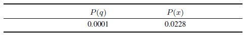
For displaying the effectiveness of algorithm,two numerical indices
are introduced.
\begin{align}%
P(q)=&\
\frac{1}{N}\sum_{i=1}^{N}(agent(i).qpre(T)-agent(i).q)^{2},\end{align}\begin{align}
P(x)=&\ \frac{1}{2N\times T}\sum_{i=1}^{N}\sum_{j=1}^{T}[(agent(i).xpre(1,j) -\\
&\ agent(i).x(1,j))^{2}+(agent(i).xpre(2,j) -\\
&\ agent(i).x(2,j)]^{2}.
\end{align}
(59)
As we can see,the indices in Table I are small compared with values of states and coupling parameters.
|
|
Table I INDICES OF DFL (SIMULATION 2) |
3) Control simulation (ContrSim)
From the above simulations,we may notice that the system without
control may not be stable due to the coupling effects even if matrix
$A_{i}$ is stable. Now we use the corresponding system with control
inputs to test the estimation effects. By the certainty equivalence
principle,control signals which regulate states to zero can be
calculated to test the estimation results. To show the effectiveness
of control design based on estimated values,we take the following
coefficient matrices and parameters:
\begin{align}%
&A_{i}=\left[\begin{array}{cc}
1&0 \\
0&1\\
\end{array}\right], \\
&C_{i}=\left[\begin{array}{cc}
0.5&0 \\
0&0.5 \\
\end{array}\right],\\
&q_{i,j_{p}}=0.6,
\end{align}
(60)
Filtering process is initialized as:
\begin{equation}
\widehat x_{i}^{*}(1)={\rm E}[x_{i}^{*}(1)],
\end{equation}
(61)
\begin{equation}%
\widehat q_{i,j_{p}}(1)=6.
\end{equation}
(62)

|
Download:
|
| Fig. 5.States comparison with or without control. | |
B.Model 2
1) Simulation 1
Consider another multi-agent system where there are $5$ agents and
every agent can be described as the following two-dimensional
dynamic model:
\begin{align}
& x_{i}(k)
=A_{i}x_{i}(k-1)+q_{i,j_{p}}x_{i-1}(k-1)+w_{i}(k-1), \\
&y_{i}(k) =C_{i}(k)x_{i}(k)+v_{i}(k).
\end{align}
(63)
\begin{align}%
&A_{i}=\left[\begin{array}{cc}
0.6&0 \\
0&0.6\\
\end{array}\right], \\
&C_{i}=\left[\begin{array}{cc}
0.8&0.7 \\
\end{array}\right],\\
&q_{i,j_{p}}=0.2,\end{align}
(64)
\begin{align}%
&\Bbb N_{i}= \left\{ \begin{array}{ll}
\{i-1\},& \textrm{if } i=2,3,4,5,\\
\{5\},& \textrm{if } i=1.\\
\end{array} \right.
\end{align}
(65)
\begin{equation}
\widehat x_{i}^{*}(1)={\rm E}[x_{i}(1)],
\end{equation}
(67)
\begin{equation}%
\widehat q_{i,j_{p}}(1)=7.
\end{equation}
(68)
Simulation results with Algorithm 2 (DFL2) are depicted in Figs. 6 $\sim$ 8. Here three agents are shown for conciseness.

|
Download:
|
| Fig. 6.Simulation 1 of Model 2: the third agent. | |

|
Download:
|
| Fig. 7.Simulation 1 of Model 2: the fourth agent. | |

|
Download:
|
| Fig. 8.Simulation 1 of Model 2: the fifth agent. | |
In every figure,the subfigure in top left corner shows the first element of states and the subfigure in bottom left corner shows the second.
2) Simulation 2
A multi-agent system with $100$ agents,each of which is the same as the above model,is chosen to verify the algorithm. Since there are many agents to be shown,to be brief,only one agent is shown in Fig. 9 and others are similar to this agent.

|
Download:
|
| Fig. 9.Simulation 2 of Model 2: the first agent. | |
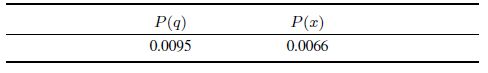
The indices in Table II are small compared with values of states and coupling parameters.
|
|
Table II INDICES OF DFL2 (SIMULATION 2) |
C.Model 3
1) Simulation 1
A multi-agent one-dimensional system with $3$ agents is chosen and
the dynamic model of every agent is given as follows:
\begin{align}
x_{i}(k)
=&-(x_{i}(k-1))^{2}+w_{i}(k-1) + \\
&\sum_{j_{p}\in\Bbb N_{i}}q_{i,j_{p}}y_{j_{p}}(k-1), \\
y_{i}(k) =&\ Cons\times(x_{i}(k))^{2}+v_{i}(k),
\end{align}
(68)
\begin{align}%
&\Bbb N_{i}= \left\{ \begin{array}{ll}
\{i-1\},& \textrm{if } i=2,3,\\
\{3\},& \textrm{if } i=1,\\
\end{array} \right.\end{align}
(69)
\begin{align}%
&w_{i}(k)\sim {\rm N}(0,Q_{i}(k)) , \\
&v_{i}(k)\sim {\rm N}(0,R_{i}(k)),
\end{align}
(70)
Filtering process is initialized as:
\begin{equation}
\widehat x_{i}^{*}(1)={\rm E}[x_{i}^{*}(1)],
\end{equation}
(71)
\begin{equation}%
\widehat q_{i,j_{p}}(1)=7.
\end{equation}
(72)
\begin{align}
\widehat P_{i}^{*}(1)={\rm E}[(x_{i}^{*}(1)-\widehat
x_{i}^{*}(1))[{x_{i}^{*}(1)-\widehat x_{i}^{*}(1)}]^{\rm T}].
\end{align}
(73)
The simulation results with Algorithm 3 (DFNL1) are depicted in Figs. 10 $\sim$ 12.

|
Download:
|
| Fig. 10.Simulation 1 of Model 3: the first agent. | |

|
Download:
|
| Fig. 11.Simulation 1 of Model 3: the second agent. | |

|
Download:
|
| Fig. 12.Simulation 1 of Model 3: the third agent. | |
Through these figures,one can see that the estimated values and the real values are nearly equal.
2) Simulation 2
A multi-agent system with $100$ agents,each of which is the same as the above model,is chosen to verify the algorithm.
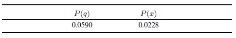
The indices in Table III are small compared with values of states and coupling parameters.
|
|
Table III INDICES OF DFNL1 (SIMULATION 2) |
D.Model 4
1) Simulation 1
A multi-agent one-dimensional system with $3$ agents is chosen and
the dynamic model of every agent is given as follows:
\begin{align}
x_{i}(k)
=&-(x_{i}(k-1))^{2}+w_{i}(k-1) + \\
&\sum_{j_{p}\in\Bbb N_{i}}q_{i,j_{p}}x_{j_{p}}(k-1), \\
y_{i}(k) =&\ Cons\times(x_{i}(k))^{2}+v_{i}(k),
\end{align}
(74)
\begin{align}%
&\Bbb N_{i}= \left\{ \begin{array}{ll}
\{i-1\},& \textrm{if } i=2,3,\\
\{3\},& \textrm{if } i=1,\\
\end{array} \right.
\end{align}
(75)
\begin{align}
w_{i}(k)\sim&\ {\rm N}(0,Q_{i}(k)), \\
v_{i}(k)\sim&\ {\rm N}(0,R_{i}(k)),
\end{align}
(76)
Filtering process is initialized as:
\begin{align}
\widehat x_{i}^{*}(1)={\rm E}[x_{i}^{*}(1)],
\end{align}
(77)
\begin{align}%
\widehat q_{i,j_{p}}(1)=6.
\end{align}
(78)
\begin{align}
\widehat P_{i}^{*}(1)={\rm E}\{[x_{i}^{*}(1)-\widehat
x_{i}^{*}(1)][{x_{i}^{*}(1)-\widehat x_{i}^{*}(1)}]^{\rm T}\},
\end{align}
(79)
The simulation results with Algorithm 4 (DFNL2) are depicted in Figs. 13 $\sim$ 15.

|
Download:
|
| Fig. 13.Simulation 1 of Model 4: the first agent. | |

|
Download:
|
| Fig. 14.Simulation 1 of Model 4: the second agent. | |

|
Download:
|
| Fig. 15.Simulation 1 of Model 4: the third agent. | |
2) Simulation 2
A multi-agent system with $100$ agents,each of which is the same as the above model,is chosen to verify the algorithm.
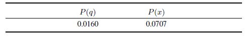
The indices in Table IV are small compared with values of states and coupling parameters.
|
|
Table IV INDICES OF DFNL2 (SIMULATION 2) |
In this contribution,we have introduced a decentralized adaptive filtering problem for a class of multi-agent systems which contain uncertain coupling parameters. This problem is important and fundamental for further studies on controlling multi-agent systems. In practice,many situations of complex systems involve such a problem since uncertain interactions are inevitable for agents,for example,nobody can successfully grow up without learning to adapt to the environment and other people. For every agent,only noisy measurement information is available,but there are uncertain interactions among agents,which make the evolution of agents become complicated and difficult to predict. The key point is to simultaneously estimate the states and unknown coupling parameters. This problem is challenging in the sense that estimating unknown coupling parameters is difficult without knowledge of precise states,and vice versa.
The considered multi-agent systems are divided into four typical types,including coupling relations which come from the effects of outputs and states of neighbor agents have on states of an agent and linear and nonlinear systems.
Then with the four typical models,decentralized filtering algorithms are deduced based on the available local information with the help of standard and extended Kalman filters by adopting the idea of states augmentation. As we can see,the modified filtering algorithms of linear systems cannot be applied directly in the nonlinear systems. And for the linear systems,modifications are made in the standard Kalman filter which need not to calculate the partial derivatives and make the calculation simple. But for the nonlinear systems,modifications are made in the extended Kalman filter. So the linear systems are not considered as the special case of the nonlinear systems. For testing the effects of estimation, decentralized adaptive controllers are designed based on certainty equivalence principle. And we provide some remarks to address the challenging issue of closed-loop stability analysis of the proposed algorithms. Then by extensive simulations,the introduced decentralized filtering algorithms have illustrated satisfactory estimation accuracy.
In the future,in-depth studies and more methods are still needed to cope with more complex situations in which influence relation among agents needs to be represented by coupling nonlinear functions. And theoretic closed-loop analysis of these methods should be conducted in detail. There is still a long way ahead along this new direction of filtering for multi-agent systems with coupling uncertainties, especially decentralized adaptive filtering of multi-agent systems with parametric coupling uncertainties as well as nonparametric coupling uncertainties.
| [1] | Yan Wei-Sheng, Li Jun-Bing, Wang Yin-Tao. Consensus for damaged multi-agent system. Acta Automatica Sinica, 2012, 38(11):1880-1884(in Chinese) |
| [2] | Yu Hong-Wang, Zheng Yu-Fan. Dynamic behavior of multi-agent systems with distributed sampled control. Acta Automatica Sinica, 2012, 38(3):357-365(in Chinese) |
| [3] | Lukomski R, Wilkosz K. Modeling of multi-agent system for power system topology verification with use of petri nets. In:Proceedings of the 2010 Modern Electric Power Systems. Wroclaw, Poland:IEEE, 2010. 1-6 |
| [4] | Ma H B, Ge S S, Lum K Y. WLS-based partially decentralized adaptive control for coupled ARMAX multi-agent dynamical system. In:Proceedings of the 2009 American Control Conference. Piscataway, NJ, United States:IEEE, 2009. 3543-3548 |
| [5] | Ma H B. Decentralized adaptive synchronization of a stochastic discretetime multi-agent dynamic model. SIAM Journal of Control and Optimization, 2009, 48(2):859-880 |
| [6] | Ma H B, Yang C G, Fu M Y. Discrete Time Systems. Vienna:I-Tech Education and Publishing, 2011. 229-254 |
| [7] | Al-Kanhal T, Abbod M. Multi-agent system for dynamic manufacturing system optimization. In:Proceedings of the 8th International Conference of Computational Science. Berlin, Germany:Springer Verlag, 2008. 634-643 |
| [8] | Luo Xiao-Yuan, Shao Shi-Kai, Guan Xin-Ping, Zhao Yuan-Jie. Dynamic generation and control of optimally persistent formation for multi-agent systems. Acta Automatica Sinica, 2013, 39(9):1431-1438(in Chinese) |
| [9] | Hall E L, Alhaj Ali S M, Ghaffari M. Engineering robust intelligent robots. In:Proceedings of the 2010 SPIE-The International Society for Optical Engineering. USA:SPIE-The International Society for Optical Engineering, 2010.753904-753918 |
| [10] | Wang P, Jiang H L, Shi W Z, Cheng M C. Design and realization of remote control in smart home system. In:Proceedings of the 2009 International Conference on Communication Software and Networks. Macau, China:IEEE, 2009. 13-15 |
| [11] | Noor A K, Venneri S L. Intelligent synthesis environment for future aerospace systems. IEEE Aerospace and Electronic Systems Magazine, 2008, 23(4):31-44 |
| [12] | Yang Z S, Sun J P, Yang C X. Multi-agent urban expressway control system based on generalized knowledge-based model. In:Proceedings of the 2003 IEEE International Conference on Intelligent Transportation Systems. Shanghai, China:IEEE, 2003. 1759-1763 |
| [13] | Kong Xiang-Jie, Shen Guo-Jiang, Sun You-Xian. Dynamic intelligent coordinated control with arterial traffic based on multi-agent. Journal of PLA University of Science and Technology (Natural Science Edition), 2010, 11(5):544-550(in Chinese) |
| [14] | Olfati-Saber R, Murray R. Consensus problems in networks of agents with switching topology and time delays. IEEE Transactions on Automatic Control, 2004, 49(9):1520-1533 |
| [15] | Ren W. Decentralization of coordination variables in multi-vehicle systems. In:Proceedings of the 2006 IEEE International Conference on Networking, Sensing and Control. Ft. Lauderdale, FL:IEEE, 2006. 550-555 |
| [16] | Ren W, Moore K, Chen Y Q. High-order consensus algorithms in cooperative vehicle systems. In:Proceedings of the 2006 IEEE International Conference on Networking, Sensing and Control. Ft. Lauderdale, FL:IEEE, 2006. 475-462 |
| [17] | Cao Y C, Ren W. Distributed containment control for multiple autonomous vehicles with double-integrator dynamics:Algorithms and experiments. IEEE Transactions on Control Systems Technology, 2011, 19(4):929-938 |
| [18] | Kalman R E. A new approach to linear filtering and prediction problems. ASME Journal of Basic Engineering, 1960, 82:34-45 |
| [19] | Simon D. Optimal State Estimation. New Jersey, America:John Wiley & Sons, Inc., 2006. |
| [20] | Wang J, Liang Q H, Liang K, Wei S Q. A new extended Kalman filter based carrier tracking loop. In:Proceedings of the 3rd IEEE International Symposium on Microwave, Antenna, Propagation and EMC Technologies for Wireless Communications. Beijing, China:IEEE, 2009. 1181-1184 |
| [21] | Wu Yao, Luo Xiong-Lin. Robustness analysis of Kalman filtering algorithm for multi-rate systems. Acta Automatica Sinica, 2012, 38(2):156-174(in Chinese) |
| [22] | Wen Tao, Ge Quan-Bo. Research on real-time block Kalman filtering estimation methods for the un-modeled system based on output measurements. Acta Electronica Sinica, 2012, 40(10):1958-1964(in Chinese) |
| [23] | Xiong Jie, Guan Wei, Sun Yu-Xing. Metro transfer passenger forecasting based on Kalman filter. Journal of Beijing Jiaotong University, 2013, 37(3):112-116, 121(in Chinese) |
| [24] | Liu Zhou-Zhou. Multi-sensor information fusion and its application. Electronic Design Engineering, 2013, 21(11):116-123(in Chinese) |
| [25] | Ma H B, Zhao Y L, Fu M Y, Yang C G. Decentralized adaptive control for a class of semi-parametric uncertain multi-agent systems. In:Proceedings of the 10th World Congress on Intelligent Control and Automation. Beijing, China:IEEE, 2012. 2060-2065 |
| [26] | Quine B M. A derivative-free implementation of the extended Kalman filter. Automatica, 2006, 42(11):1927-1934 |
| [27] | Jazwinski A J. Stochastic Process and Filter Theory. New York:Academic Press, 1970. |
| [28] | Solo V. Stability of the Kalman filter with stochastic time-varying parameters. In:Proceedings of the 35th IEEE Conference on Decision and Control. Kobe, Japan:IEEE, 1996. 57-61 |
| [29] | Reif K, Gunther S, Yaz E, Unbehauen R. Stochastic stability of the discrete-time extended Kalman filter. Automatic Control, 1999, 44(4):714-728 |