I. INTRODUCTION

Study of multi-agent systems (MAS) is concerned with the development and analysis of control architectures and sophisticated artificial intelligence problem-solving for both single- and multiple-agent systems. A typical topic of research in MAS is the multi-vehicle cooperative formation control problem, which is to control the displacement and/or attitude of each vehicle within some workspace to accomplish a common task. Since a vehicle can be considered as an actual implementation of an agent, the word "vehicle" in this paper will be equivalent to the word "agent".

It can be argued that a group of vehicles can perform tasks faster and more efficiently compared to a single vehicle. For example,a group of robots can be employed to move a large object which may be difficult or impossible for a single robot; multiple unmanned aerial vehicle (UAV) and autonomous underwater vehicle (AUV) formations achieve better area coverage for reconnaissance,thereby improving mission success^[1]. In recent years,research in cooperative flight control of multi-aircraft systems has attracted growing interest. The implications of the formation flight are very significant,not just for fuel and energy saving but for future applications across civilian and military domains^[2]. For instance,formation flight can be used to handle the increase in air traffic around airports by means of civil aeroplane formations taking-off and landing to improve the efficiency of runway use. Applications in the military field include aerial refueling, include aerial refueling,aircraft logistics,air formation systems.

More specifically,there are four cooperative formation control strategies of importance: behaviour-based strategy, leader-following approach,virtual structure method and artificial potential field approach.

The behaviour-based approach is decentralised and the control action of each element in the formation is a weighted average of the control for each behaviour^[3]. Its main advantage is that the collision avoidance problem can be easily dealt with due to the existing reactions between vehicles. However,the whole system is more complex and difficult to be analysed mathematically.

In the leader-following approach^[4],some vehicles are considered as leaders,while others act as followers. The leader vehicle maintains the given trajectory while the followers track a fixed relative distance from the designated neighbouring vehicles^[5]. This technique is decentralised,conceptually simple and widely employed in multi-vehicle formation control. Its major drawback is that the leader becomes a single point of failure,as well as producing error propagation that incurs poor responses for the followers.

The virtual structure approach is centralised and describes the whole formation as a single rigid body^[6]. Each vehicle has its own relative position in the body and tracks the desired trajectory which is translated from the desired motion of the rigid body^[7]. Its strength is that all elements in the formation hold the same transient without error propagation,and a tight formation can then be implemented and maintained. However, it contains a single point of failure which is undesirable,since collision avoidance is not possible due to the absence of interaction between the vehicles,as well as a lack of explicit feedback to the formation.

The standard artificial potential field approach is based on applying the negative gradient of an artificial potential function (APF) as control inputs to drive the overall formation to convergence^[8]. This technique is decentralised,reactive, and can be beneficially combined with the behaviour-based method to make use of both benefits. However,it suffers from a problem with local minima and there is computational difficulty in designing a feasible artificial potential function.

1) Stability analysis approach

Any closed-loop formation control methodology must naturally be guaranteed to be stable,especially where there is a potential of loss of human life and property. Most research papers in this area make use of either algebraic graph theory or Lyapunov stability theory.

The use of graph theory in the analysis of interconnected systems is not new,and the current interest is in applying graph-theoretic concepts to the multi-vehicle formation problem. An application of graph theory was discussed in ^[9],where a directed graph was used to represent the \hfill communication network and to relate its topology with forma tion stability. Desai et al. in ^[10] presented a framework for describing the behaviours of robots in a formation,representing possible control graphs and the coordination of transitions with formation changes from one geometry to another. Additionally,in ^[11],elementary graph theory and linear matrix inequalities (LMI) were combined with logic-based switching to shed light on the various control strategies which are feasible in the leader-following framework for formation flying of multiple spacecraft. Furthermore,graphs have also been applied to describe the interconnection topology in a formation^[12],to reflect the control structure, information flow,and error propagation.

Lyapunov stability theory is an alternative way to analyse the overall formation stability. In ^[13],a formation Lyapunov stability function was defined as a weighted sum of the control Lyapunov function for each vehicle to support the formation stability analysis. In ^[8],the idea of relative-position-based formation stability was proposed and the Lyapunov method was also used to design the decentralised controllers,along with an extended LMI to analyse the conditions required for formation stability. Moreover, Hong et al. in ^[14] proposed a Lyapunov-based approach to give a sufficient condition to make all the agents converge to a common value,and a common Lyapunov function was explicitly constructed in the case of switching jointly connected topologies. In another paper^[15],a combination of the above two strategies was employed,where a few concepts from graph theory were borrowed to evaluate the controllability and observability of the individual system and a vector Lyapunov method was then applied to prove the stability of the multi-vehicle formation.

2) Contribution of this paper

The purpose of this paper is to propose a formation stability conjecture which is used to conceive a new methodology for decentralised multi-vehicle formation control and to analyse its associated formation stability. Although differing from the previous strategies,it necessarily builds on them and has the desired characteristics.

Based on the formation stability conjecture,the "extension-decomposition-aggregation (EDA)" process^[16] is adopted to support the decentralised formation controller design and formation stability analysis. A virtual additional system (VAS) is first employed to build the relationship between isolated vehicles and to produce an overall formation control system involving formation information. Decomposition to the overall formation system is then carried out to translate this complex formation system into a group of feasible subsystems interacting via boundary conditions. These decomposed subsystems are referred to as individual augmented subsystems (IASs). A scalar Lyapunov function is next selected as an index for representing the stability of each IAS. These indices are finally aggregated to analyse the subsystem interactions and the stability of the overall formation using Lyapunov theory. It is concluded that the overall formation system is not only asymptotically but also exponentially stable in the sense of Lyapunov within a neighbourhood of the desired formation,if all the IASs can be stabilised by using any approach. It is essential to note that the proposed methodology on multi-vehicle formation control and stability analysis in this paper can be easily extended into research of other topic in multi-agent system.

The remainder of the paper is organised as follows. Section II outlines the problem formulation. Section~III presents the formation stability conjecture and its specific EDA scheme,whilst Section~IV describes the relevant stability analysis of the overall formation system. Extensive simulation results are presented in Section V to illustrate the feasibility and verify the formation stability. The paper finally concludes with some discussion and suggestions for future work.

II. PROBLEM FORMULATION

It is essential to note that only using the formation geometry between the vehicles is not sufficient to define a formation,since the motion of each vehicle in 3-D space has six DOF defining the position and attitude,and unstable attitude will definitely affect the above relative distance. On the other hand,it is believed that when a formation change is needed,the related attitude should generally be regulated by a formation control algorithm until all the vehicles achieve their new desired formation geometry. In other words,the primary function of formation controller is to maintain the stability of the relative positions by controlling the {states} of each vehicle (such as aircraft attitude angles).

Motivated by this,a complete formation definition (FD) in Euclidean space should consist of the relative distances,and states of all the vehicles. Here,$\tilde{\pmb{x}}_{i}$ is to denote the state of the $i$th vehicle,whilst the overall state of the formation system with $N$ vehicles is defined as a vector $\tilde{\pmb{x}}$ $=$ $[\tilde{\pmb{x}}_{1};\tilde{\pmb{x}}_{2}; \cdots; \tilde{\pmb{x}}_i; \cdots; \tilde{\pmb{x}}_{N}]$ by combining the states of all the individual vehicles. Taking these into account, the FD is expressed as (1) in terms of the relative distances and each vehicle$'$s states.

\begin{align}\label{eq:formaDefine2} \begin{split} {\rm FD}: {\kern 12pt} &F_{\rm real}=\{{{\pmb{r}}_{ij}}:i,j = 1,\cdots ,N;i \ne j\},\\ &{{\tilde{\pmb{x}}}}=[\tilde{\pmb{x}}_{1};\tilde{\pmb{x}}_{2}; \cdots; \tilde{\pmb{x}}_i; \cdots; \tilde{\pmb{x}}_{N}], \end{split} \end{align}

(1)

where the subscript "real" represents the real-time formation,and "$\pmb{r}_{ij}$" means relative distance between the $i$th vehicle and the $j$th vehicle.

Similar to the state definition $\tilde{\pmb{x}}$ of the overall formation system,the input vector of the overall formation system is defined as $\tilde{\pmb{u}}=[\tilde{\pmb{u}}_{1};\tilde{\pmb{u}}_{2}; \cdots; \tilde{\pmb{u}}_i; \cdots; \tilde{\pmb{u}}_{N}]$ which consists of input vectors of all the individual vehicles. Based on the above definitions,a common and intuitive definition to formation stability is now presented below.

${\bf Formation stability definition 1.}$ The formation with $N$ vehicles is asymptotically stable in the sense of Lyapunov if the following is satisfied^[1],

\begin{equation}\label{eq:FormaCommDef} \mathop {\lim }\limits_{t \to + \infty } \left\| {{L(\tilde{\pmb{x}},\tilde{\pmb{u}})} - {{L}_{e}}} \right\| = 0,\\ \end{equation}

(2)

where $t$ is the elapsed time,$L(\tilde{\pmb{x}},\tilde{\pmb{u}})$ defined by (3) is called cumulative formation error,and denotes the summation over the individual formation errors. $L_{e}$ represents the equilibrium value of $L(\tilde{\pmb{x}},\tilde{\pmb{u}})$,and from the viewpoint of an optimisation problem,$L_{e}$ should be the minimum of $L(\tilde{\pmb{x}},\tilde{\pmb{u}})$,i.e.,$L_{e} = \min\{L(\tilde{\pmb{x}},\tilde{\pmb{u}})\}$.

\begin{equation}\label{eq:FormaLengDef} L(\tilde{\pmb{x}},\tilde{\pmb{u}}) = \sum\limits_{i = 1}^N {\sum\limits_{j = 1,j \ne i}^N {\left( {{L_{i \leftarrow j}}({\tilde{\pmb{x}}_{i}},{\tilde{\pmb{x}}_{j}}) + {{\left\| {{\tilde{\pmb{u}}_{i}}} \right\|}^2}} \right)} }. \end{equation}

(3)

In (3),${{L_{i \leftarrow j}}({\tilde{\pmb{x}}_{i}},{\tilde{\pmb{x}}_{j}})}$ is a cost function and represents the individual formation error between the $i$th vehicle and $j$th vehicle,and the final term ${{\left\| {{\tilde{\pmb{u}}_{i}}} \right\|}^2}$ is a penalty on the inputs.

It is obvious that the above definition illustrates the formation stability from a global perspective,but may not be convenient for analysing the stability of the decentralised formation control strategy. Here,based on the formation definition in (1),another definition is given as follows.

${\bf Formation stability definition 2.}$ The formation with $N$ vehicles is asymptotically stable in the sense of Lyapunov if the followings are satisfied,

\begin{align} \label{eq:FormaStableDef1} &\mathop {\lim }\limits_{t \to + \infty } \left\| {{F_{\rm real}} - {F_{e}}} \right\| = 0,\end{align}

(4)

\begin{align} \label{eq:FormaStableDef2} &\mathop {\lim }\limits_{t \to + \infty } \left\| {{\tilde{\pmb{x}}} - {\tilde{\pmb{x}}_{e}}} \right\| = 0, \end{align}

(5)

where $t$ is the elapsed time,$F_{e}$ indicates the equilibrium shape of the overall formation,and $\tilde{\pmb{x}}_{e} = [\tilde{\pmb{x}}_{e_1};\tilde{\pmb{x}}_{e_2}; \cdots; \tilde{\pmb{x}}_{e_N}]$ consists of the equilibrium states of $\tilde{\pmb{x}}_i$,$i=1,2,\cdots,N$. This formation stability definition means that both the states of all the vehicles and the relative distances between them should converge to steady states.

It is obvious that $F_{\rm real}$ in (4) shows a global expression of the overall formation. Based on the adopted decentralised control architecture,it is assumed that $F_{\rm real}$ can be decomposed into a set of local-formation representations,i.e.,

\begin{equation} \label{eq:FormaDecom} F_{\rm real} = \{F_{\rm real_1},F_{\rm real_2},\cdots,F_{ {\rm real}_i},\cdots,F_{{\rm real}_N}\} \end{equation}

(6)

where $F_{{\rm real}_i}$ corresponds to the local-formation representation of the $i$th vehicle. Suppose that it can be expressed by a vector $\pmb{x}_{F_{{\rm real}_i}}$ to reflect the variation of the associated local-formation. The state vector $\tilde{\pmb{x}}_{i}$ of the $i$th vehicle can then be augmented as

\begin{align} \label{eq:AugmState} {\pmb x}_{i}=[\tilde{\pmb{x}}_{i}^{\rm T},{\pmb x}_{F_{{\rm real}_i}}^{\rm T}]^{\rm T}, \end{align}

(7)

where ${\pmb x}_{i}$ is considered as the augmented state vector derived from the original one,$\tilde{\pmb {x}}_{i}$ of the $i$th vehicle. Based on this,formation stability definition 2 is then redefined as follows.

${\bf Formation stability definition 3.}$ The formation with $N$ vehicles is asymptotically stable in the sense of Lyapunov if the following is satisfied,

\begin{equation} \label{eq:FormaStableSim} \mathop {\lim }\limits_{t \to + \infty } \left\| {{\pmb X} - {{\pmb X}_{e}}} \right\| = 0,\\ \end{equation}

(8)

where ${\pmb X}=[{{\pmb x}}_{1}; {\pmb {x}}_{2}; \cdots; {\pmb{x}}_{i}; \cdots; {\pmb{x}}_{N}]$ consists of all the state vectors of the augmented systems derived from the original vehicle systems,and ${{\pmb X}_{e}}=[{\pmb{x}}_{e_1}; {\pmb{x}}_{e_2}; \cdots; {\pmb{x}}_{e_i}; \cdots; {\pmb{x}}_{e_N}]$ denotes the equilibrium states including all the individual equilibrium states of the augmented systems. Although the above three definitions show different forms,they are equivalent to each other in essence.

III. NOVEL FORMATION CONTROL STRATEGY

Most formation control approaches mentioned previously are direct methods and are based on direct distance or position errors. Such methods are easy to understand,but are not necessarily suitable for analysing and implementing a practical formation control system. Here,a formation stability conjecture is proposed to conceive a new methodology for dealing with multi-vehicle decentralised formation control problem.

A.Formation Stability Conjecture

As to the problem of formation control of multiple vehicles,it is obvious that ensuring the stability of all the original vehicles in a formation is not sufficient to prove the stability of the overall formation because equation (4) cannot be guaranteed. However,are there corresponding augmented systems from the original vehicles to support the analysis of formation stability? If the answer is yes and the stability of all the augmented systems is able to guarantee the stability of the overall formation system,the process of solving the formation control problem can be greatly simplified. Hence,motivated by this idea,we propose a conjecture as follows:

${\bf Formation stability conjecture.}$ The overall formation system is guaranteed to be stable if the following three requirements are satisfied.

1) There exists a group of dynamic systems \textnormal{(DSs)} which are augmented from corresponding original vehicles.

2) All the \textnormal{DSs} interacting with each other completely constitute the overall formation control system.

3) Each individual \textnormal{DS} can be stabilised by the respective decentralised controller.

The relationship between the conjecture and the analysis of the formation stability is intuitively given in Fig. 1,where stage 1 will be discussed in Section \ref{StabilityAnaly},the stage 2 is supported by the formation stability definition 3. It is essential to point out that the DS represents a system that needs to be determined or designed. Recalling the definition of the augmented states in (8),a DS can be considered as the augmented system of each original vehicle,and the combination of states of all the DSs can also be denoted by ${\pmb X}=[{\pmb{x}}_{1}; {\pmb{x}}_{2}; \cdots; {\pmb{x}}_{i}; \cdots; {\pmb{x}}_{N}]$,where $\pmb{x}_{i}$ means the augmented state vector of the $i$th DS. If all the DSs can be stabilised by their decentralised controller,it means that the stability requirement in (\ref{eq:FormaStableSim}) is guaranteed,and consequently the whole formation system is stable.

Based on the proposed conjecture,the analysis process of the overall formation stability can be briefly listed as the following procedure:

${\bf Step 1.}$ Attempt to seek or determine feasible DSs according to a desired specification.

${\bf Step 2.}$ Design individual controllers to stabilise all the achieved DSs.

${\bf Step 3.}$ Carry out simulation analyses to verify the performance of the overall formation system. If the achieved performance is not satisfied with the desired target,return to Step 1.

${\bf Step 4.}$ If the performance in Step 3 is satisfactory, analyse the stability of the whole formation mathematically.

In the above descriptions,the determination of the DSs is the strategic point,and the stability of the overall formation is completely dependent on them. In other words,if the suitable DSs are found,mathematical stability analysis and implementation of the decentralised formation controller become feasible and convenient.

Based on the above conjecture and the subsequent procedure,the "extension-decomposition-aggregation (EDA)" proposed in ^[16] is considered as an implementation of the formation stability conjecture. In contrast to ^[16],this paper focuses on mathematically analyzing the stability of multi-vehicle formation based on this EDA. This will be discussed in the next subsection.

B.Extension-decomposition-aggregation Strategy for Formation Control

The design framework of the EDA scheme is illustrated in Fig. 2. The introduced virtual additional system (VAS) is: 1) to build a relationship between the isolated vehicles,leading to a new overall formation control system; 2) to involve the desired formation variables or parameters,which could be combined with the related individual vehicle model; 3) to support the subsequent decomposition,and simplify the stability analysis to the overall formation.

Note that the VAS is merely an algorithm to act as an "interaction bridge" providing each vehicle with the capability of sensing its local-formation states,which can then be used for the formation controller design.

Since the overall formation system involving many variables is difficult to handle as a whole,it is natural to decompose it into several local-formation subsystems. However,it should be noted that there is no general systematic procedure for decomposing such a complex dynamical control system. Here,using physical insight, the overall formation system is decomposed into $N$ individual subsystems,each being called individual augmented subsystem (IAS) since it combines the individual vehicle model and the local-formation variables.

In light of the above definitions and descriptions,the procedure for analysing the whole formation stability is specified as follows:

1) All the decomposed subsystems or IASs are used to design the decentralised formation controllers,the interactions between them being considered as the bounded exogenous disturbances.

2) The formation stability of each vehicle,involving several state variables,is represented by a single variable --- the Lyapunov function (say,$V_i$ for $i$th vehicle),which is considered as an index for each subsystem representing local-formation stability. This approach simplifies the stability problem,although it sacrifices the detailed information about the size of variation of each separate state variable.

3) These indices ($V_i$,$i=1,2,\cdots,N$) are aggregated and the interactions between them are studied to analyse mathematically the stability of the overall formation,neglecting the interconnections between decomposed subsystems.

Broadly speaking,the $N$ IASs are associated with the $N$ scalar Lyapunov functions ($V_i$,$i=1,2,\cdots,N$),and each determines the stability property of an individual IAS. These scalar functions are considered as the components of the overall Lyapunov function $V$. A differential inequality is formed in terms of this function, using the original inequalities of the decomposed IASs. The stability of the overall formation control system can then be determined by considering only the differential inequalities involving the $N$ Lyapunov functions. This brings about a considerable reduction in the dimensionality of the formation stability problem.

IV. FORMATION STABILITY ANALYSIS

Recalling the EDA scheme shown in Fig. 2, the coupled multiple pendulum (CMP)^[17] system is suitable to be considered as a candidate of the VAS,where the variation of $\varepsilon_i$ is a reflection of the formation error,and there also exists an important equation expressed as (9)^[18]

\begin{equation}\label{eq:SumMeshTor} \sum\limits_{j=1,j\neq 1}^{N}{{T_{1j}}} + \sum\limits_{j=1,j\neq 2}^{N}{{T_{2j}}} + \cdots + \sum\limits_{j=1,j\neq N}^{N}{{T_{Nj}}} = 0, \end{equation}

(9)

where $T_{ij}$ denotes the torque on the $i$th pendulum exerted by the interacting $j$th pendulum. The achieved equations above crucially show that if all the individual pendulums are stable, the resultant torque of the whole CMP is equal to zero whatever the interconnection formation topology is. This useful result can be used to support the overall formation stability analysis of the multi-vehicle formation.

It is assumed that the overall formation control system,$S$ consisting of the CMP system as the VAS,can be linearised and decomposed into $N$ coupled subsystems or so-called IAS, ${\pmb{S}}_i$ $(i=1,2,\cdots,N)$ as

\begin{equation} \label{eq:OverallSysL} {\pmb{S}}:{\kern 8pt} \left\{ {\begin{array}{*{20}{l}} {{{\pmb{S}}_1}:{{{\dot{\pmb x}}}_1} = {A_1}{{\pmb{x}}_1} + {h_{12}}(t,{{\pmb{x}}_2})},\\ {{{\pmb{S}}_2}:{{{\dot{\pmb x}}}_2} = {A_2}{{\pmb{x}}_2} + {h_{21}}(t,{{\pmb{x}}_1}) + {h_{23}}(t,{{\pmb{x}}_3})},\\ \qquad\qquad\quad \vdots \\ {{{\pmb{S}}_i}:{{{\dot{\pmb x}}}_i} = {A_i}{{\pmb{x}}_i} + {h_{i(i-1)}}(t,{{\pmb{x}}_{i - 1}}) + {h_{i(i+1)}}(t,{{\pmb{x}}_{i + 1}})},\\ \qquad\qquad\quad \vdots \\ {{{\pmb{S}}_N}:{{{\dot{\pmb x}}}_N} = {A_N}{{\pmb{x}}_N} + {h_{N(N-1)}}(t,{{\pmb{x}}_{N-1}})}, \end{array}} \right. \end{equation}

(10)

where ${h_{i(i-1)}}(t,{{\pmb{x}}_{i-1}})$ and ${h_{i(i+1)}}(t,{{\pmb{x}}_{i+1}})$ describe the interactions of the $i$th IAS with its neighbouring $(i-1)$th and $(i+1)$th IASs, respectively. Now consider the stability of the corresponding decoupled linear time-invariant subsystems $\tilde{\pmb{S}}_1, \tilde{\pmb{S}}_2,\cdots,\tilde{\pmb{S}}_N$ by ignoring the above interactions.

\begin{align} \label{eq:DecomSysL} \begin{split} &\tilde{\pmb{S}}_1:{{{\dot{\pmb x}}}_1} = {A_1}{{\pmb{x}}_1},\\ &\tilde{\pmb{S}}_2:{{{\dot{\pmb x}}}_2} = {A_2}{{\pmb{x}}_2},\\ &\qquad\qquad \vdots \\ &\tilde{\pmb{S}}_N:{{{\dot{\pmb x}}}_N} = {A_N}{{\pmb{x}}_N}. \end{split} \end{align}

(11)

For the stability of $\tilde{\pmb{S}}_i$ in (11), a scalar function

\begin{equation} \label{eq:DecomLyap} {{V}_i}({{\pmb{x}}_i}) = ({\pmb{x}}_i^{\rm T}{P_i}{{\pmb{x}}_i})^{\frac{1}{2}},\ i=1,2,\cdots ,N, \end{equation}

(12)

is defined as a candidate Lyapunov function. Thus,for any choice of the positive definite matrices $Q_i$,there exist positive definite matrices $P_i$ as the solution to the Lyapunov matrix equation (13).

\begin{equation} \label{eq:LyaEquL} A_i^{\rm T}{P_i} + {P_i}{A_i} = -{Q_i}. \end{equation}

(13)

The time derivative of the function ${{V}_i}({\pmb{x}}_i)$ along the solution of subsystem $\tilde{\pmb{S}}_i$ is therefore given by

\begin{equation} \label{eq:LyaDerivL} {{\dot{V}}_i} = {(grad{\kern 6pt}{V_i})^{\rm T}}{{{\dot{\pmb x}}}_i} = {(grad{\kern 6pt}{V_i})^{\rm T}}{A_i}{{\pmb{x}}_i} = -{\frac{1}{2}}{{V}_i}^{-1}({\pmb{x}}_i^{\rm T}{Q_i}{{\pmb{x}}_i}), \end{equation}

(14)

where $(grad{\kern 6pt}{{V}_i})={{V_i}^{-1}}{P_i}{\pmb{x}}^{\rm T}_i$. From the above equations,the range estimates for ${V}_i({\pmb{x}}_i)$,${\dot{V}}_i({\pmb{x}}_i)$ and $\left\| {grad{\kern 6pt}{{V}_i}} \right\|$ are given by^[19]

\begin{equation} \label{eq:EstimateL} \left\{ \begin{array}{l} {c_{i1}}\left\| {{{\pmb{x}}_i}} \right\| \le {{V}_i}({{\pmb{x}}_i}) \le {c_{i2}}\left\| {{{\pmb{x}}_i}} \right\|,\\[1mm] {{\dot{{V}}}_i}({{\pmb{x}}_i}) \le -{c_{i3}}\left\| {{{\pmb{x}}_i}} \right\|,\\[1mm] \left\| {grad{\kern 6pt}{{V}_i}} \right\| \le {c_{i4}}, \end{array} \right.{\kern 5pt} i = 1,2,\cdots ,N, \end{equation}

(15)

where

\begin{equation} \label{eq:EstiParamL} \begin{array}{ll} {c_{i1}} = \lambda_m^{\frac{1}{2}}({P_i}),&{c_{i2}} = \lambda _M^{\frac{1}{2}}({P_i}),\\[2mm] {c_{i3}} = \dfrac{1}{2}\dfrac{{{\lambda _m}({Q_i})}}{{\lambda_M^{\frac{1}{2}}({P_i})}},& {c_{i4}} = \dfrac{{{\lambda_M}({P_i})}}{{\lambda_m^{\frac{1}{2}}({P_i})}}, \end{array} \end{equation}

(16)

and the properties of a positive semi-definite symmetric matrix ($H$) shown in (17) and (18) are used in achieving (16),

\begin{align} \label{eq:UsefulProp} &\lambda_m(H){\pmb{x}}^{\rm T}{\pmb{x}} \le {\pmb{x}}^{\rm T}H{\pmb{x}} \le \lambda_M(H){\pmb{x}}^{\rm T}{\pmb{x}},\end{align}

(17)

\begin{align} \label{eq:UsefulProp2} &{\pmb{x}}^{\rm T}{\pmb{x}} = {\left\| {{{\pmb{x}}_i}} \right\|}^2, \end{align}

(18)

where $\lambda_M$ and $\lambda_m$ are the maximum and minimum eigenvalues of the indicated matrix,respectively. Note that the coefficients $c_{i1}$,$c_{i2}$,$c_{i3}$,and $c_{i4}$ are positive because of the positive definite property of matrices $P_i$ and $Q_i$.

Now the Lyapunov function ${{V}}_i({\pmb{x}}_i)$ is used as the stability index for each linear subsystem $\tilde{\pmb{S}}_i$. Furthermore,the derivative ${\dot{V}}_i$ along the solutions of the interacting IAS (${\pmb{S}}_i$) in (10) is given by

\begin{align} \label{eq:LyaDerivConnL} {{\dot{V}}_i} =&\ {(grad{\kern 3pt}{{V}_i})^{\rm T}}{{{\dot{\pmb x}}}_i} =\notag\\ &\ {(grad{\kern 3pt}{{V}_i})^{\rm T}}[{A_i}{{\pmb{x}}_i}\!+ {h_{i(i-1)}}(t,{{\pmb{x}}_{i - 1}}) \!+ {h_{i(i+1)}}(t,{{\pmb{x}}_{i + 1}})]\!=\notag\\ &\ {(grad{\kern 3pt}{{V}_i})^{\rm T}}{A_i}{{\pmb{x}}_i} + {(grad{\kern 3pt}{{V}_i})^{\rm T}}[{h_{i(i-1)}}(t,{{\pmb{x}}_{i - 1}}) +\notag\\ &\ {h_{i(i+1)}}(t,{{\pmb{x}}_{i + 1}})]. \end{align}

(19)

Note that the first term,${(grad{\kern 3pt}{{V}_i})^{\rm T}}{A_i}{{\pmb{x}}_i}$,is associated with the decoupled system (11),and the expression,$\| {{{\pmb{x}}_i}} \| \ge c_{i2}^{ - 1}{{V}_i}({{\pmb{x}}_i})$,follows from the first inequality in (15). So,there exists an inequality given by

\begin{equation} \label{eq:LyaDerivEvaL} \begin{array}{l} {(grad{\kern 3pt}{{V}_i})^{\rm T}}{A_i}{{\pmb{x}}_i} \le - {c_{i3}}\left\| {{{\pmb{x}}_i}} \right\| \le -{c_{i3}}c_{i2}^{-1}{{V}_i}. \end{array} \end{equation}

(20)

The stability of the overall formation system,$\pmb{S}$,is expressed by considering the interactions between these ${{V}}_i({\pmb{x}}_i)$,$i=1,2,\cdots,N$. The function given in (21) defines the Lyapunov function $\pmb{V}$ for $\pmb{S}$,which is the weighted sum of all the individual Lyapunov functions,${{V}}_i({\pmb{x}}_i)$,$i= 1,2$,$\cdots$,$N$,

\begin{align} \label{eq:OverallLyaL} {\pmb{V}} = &\ \sum\limits_{i=1}^N {{k_i}}{V_i}({{\pmb{x}}_i}) =\nonumber\\ &\ {k_1}{V_1}({{\pmb{x}}_1}) + {k_2}{V_2}({{\pmb{x}}_2}) + \cdots + {k_N}{V_N}({{\pmb{x}}_N}), \end{align}

(21)

where the choice of coefficients ${k_i}$,$i=1,2,\cdots,N$ reflects that vehicles in a formation may have completely different dynamics. Its time derivative $\dot{\pmb{V}}$ is given as

\begin{align} \label{eq:OverallLyaDerivL} \dot{\pmb{V}} &= {k_1}{{\dot V}_1}({{\pmb{x}}_1}) + {k_2}{{\dot V}_2}({{\pmb{x}}_2}) + {k_3}{{\dot V}_3}({{\pmb{x}}_3}) + \cdots + {k_N}{{\dot V}_N}({{\pmb{x}}_N})=\notag\\ & {\kern 8pt} \sum\limits_{i=1}^N {{k_i}}{(grad{\kern 6pt}{{V}_i})^{\rm T}}{A_i}{{\pmb{x}}_i}+ [0+{(grad{\kern 5pt}{{V}_1})^{\rm T}}{k_1}{h_{12}}(t,{{\pmb{x}}_2})] +\notag\end{align}\begin{align} & {\kern 8pt} [{(grad{\kern 5pt}{{V}_2})^{\rm T}}{k_2}{h_{21}}(t,{{\pmb{x}}_1})+{(grad{\kern 5pt}{{V}_2})^{\rm T}}{k_2}{h_{23}}(t,{{\pmb{x}}_3})] +\notag\\ & {\kern 9pt} [{(grad{\kern 5pt}{{V}_3})^{\rm T}}{k_3}{h_{32}}(t,{{\pmb{x}}_2})+ {(grad{\kern 5pt}{{V}_3})^{\rm T}}{k_3}{h_{34}}(t,{{\pmb{x}}_4})] + \notag\\ & {\kern 8pt} \cdots + {(grad{\kern 5pt}{{V}_{N-1}})^{\rm T}}{k_{N-1}}{h_{(N-1)N}}(t,{{\pmb{x}}_N})] +\notag\\ & {\kern 8pt} [{(grad{\kern 5pt}{{V}_N})^{\rm T}}{k_{N}}{h_{N(N-1)}}(t,{{\pmb{x}}_{N-1}})+0]. \end{align}

(22)

By taking the norm on the right-hand side of (22) and using the estimates in (15) and (20),the $\dot{\pmb{V}}$ is then given

\begin{align} \label{eq:OverLyaDeriv2L} \dot{\pmb{V}} \le & \sum\limits_{i=1}^N (-{{c_{i3}}c_{i2}^{-1}}k_i{V_i})\! + \nabla_{\max}k_{\max}[{h_{12}}(t,{{\pmb{x}}_2})\! + {h_{21}}(t,{{\pmb{x}}_1}) +\notag\\ & \ {h_{23}}(t,{{\pmb{x}}_3}) + {h_{32}}(t,{{\pmb{x}}_2})+ {h_{34}}(t,{{\pmb{x}}_4})+ \cdots +\notag\\ & \ {h_{(N-1)N}}(t,{{\pmb{x}}_N}) + {h_{N(N-1)}}(t,{{\pmb{x}}_{N - 1}})] \le\notag\\ & -c_{\min}({k_1}{V_1}+{k_2}{V_2} + {k_3}{V_3} + \cdots + {k_N}{V_N}) +\notag\\ & \ \nabla_{\max}k_{\max}[{h_{12}}(t,{{\pmb{x}}_2}) + {h_{21}}(t,{{\pmb{x}}_1}) + {h_{23}}(t,{{\pmb{x}}_3}) +\notag\\ & \ {h_{32}}(t,{{\pmb{x}}_2})+ \cdots + {h_{(N-1)N}}(t,{{\pmb{x}}_N}) +\notag\\ & \ {h_{N(N-1)}}(t,{{\pmb{x}}_{N - 1}})] , \end{align}

(23)

where $k_{\max}$ $=$ $\max\{k_1$,$k_2$,$\cdots$,$k_N\}$, $\nabla_{\max}=\max\{ \left\| (grad{\kern 5pt}{{V}_1})^{\rm T} \right\|$,$\left\| (grad{\kern 5pt}{{V}_2})^{\rm T} \right\|$, $\cdots$,$\left\| (grad{\kern 5pt}{{V}_N})^{\rm T} \right\| \}$ and $c_{\min} = \min\{c_{13}c_{12}^{-1},c_{23}c_{22}^{-1},\cdots, c_{N3}c_{N2}^{-1}\}>0$.

Moreover,depending on the characteristics of the CMP,the interaction terms,$h_{ij}$,$i\neq j$,$i,j=1,2,\cdots,N$ in the model of (11) correspond to the torques of the CMP system. The result achieved in (9) can be used to generate the following equation:

\begin{align} \label{eq:SumInteractL} &{h_{12}}(t,{{\pmb{x}}_2})+{h_{21}}(t,{{\pmb{x}}_1})+{h_{23}}(t,{{\pmb{x}}_3})+{h_{32}}(t,{{\pmb{x}}_2})+ \cdots +\notag\\ &\qquad {h_{(N-1)N}}(t,{{\pmb{x}}_N})+{h_{N(N-1)}}(t,{{\pmb{x}}_{N - 1}})=0. \end{align}

(24)

If all the decomposed IASs can be stabilised,these terms satisfy the condition in (\ref{eq:SumInteractL}). By incorporating (\ref{eq:SumInteractL}) in (\ref{eq:OverLyaDeriv2L}),the following differential inequality is obtained.

\begin{align} \label{eq:DiffInequL} \dot{\pmb{V}} \le & -{c_{\min}}[{k_1}{V_1}({{\pmb{x}}_1}) + {k_2}{V_2}({{\pmb{x}}_2}) + \cdots + {k_N}{V_N}({{\pmb{x}}_N})] =\notag\\ & -c_{\min}V. \end{align}

(25)

The above inequality is valid for all $t \ge t_0$,and its solution is given by

\begin{equation} \label{eq:RootsL} \pmb{V} \le {\pmb{V}_0}\exp [-c_{\min}(t-{t_0})],{\kern 8pt} t \ge {t_0}, \end{equation}

(26)

where ${\pmb V}_0={k_1}V_{10}+{k_2}V_{20}+ \cdots +{k_N}V_{N0}$ is the initial value of $\pmb{V}$ for the overall formation system,and $V_{10},V_{20},\cdots,V_{N0}$ denote the initial values corresponding to the subsystems $({\pmb{S}}_i$,$i=1,2,\cdots, N)$. Then,using the first inequality in (15) for the functions $V_1({\pmb{x}}_1),V_2({\pmb{x}}_2),\cdots, V_N({\pmb{x}}_N)$,as well as the definition (21), the following inequalities hold,

\begin{align} \label{eq:EstimInequL} {\pmb V} \ge&\ {k_1}c_{11}\left\| {{{\pmb{x}}_1}} \right\| + {k_2}c_{21}\left\| {{{\pmb{x}}_2}} \right\| + \cdots + {k_N}c_{N1}\left\| {{{\pmb{x}}_N}} \right\|\ge \notag\\ &\ {c_{m}}\left( {\left\| {{{\pmb{x}}_1}} \right\| + \left\| {{{\pmb{x}}_2}} \right\| + \cdots + \left\| {{{\pmb{x}}_N}} \right\|} \right),\notag\\ {\pmb{V}_0} \le&\ {k_1}c_{12}\left\| {{{\pmb{x}}_{10}}} \right\| + {k_2}c_{22}\left\| {{{\pmb{x}}_{20}}} \right\| + \cdots + {k_N}c_{N2}\left\| {{{\pmb{x}}_{N0}}} \right\| \le\notag\\ &\ {c_{M}}\left( {\left\| {{{\pmb{x}}_{10}}} \right\| + \left\| {{{\pmb{x}}_{20}}} \right\| + \cdots + \left\| {{{\pmb{x}}_{N0}}} \right\|} \right), \end{align}

(27)

where $c_{m}$ $=$ $\min\{{k_1}c_{11}$,${k_2}c_{21}$,$\cdots$, ${k_N}c_{N1}\}$ $>$ $0$,$c_{M}=\max\{{k_1}c_{12}$,${k_2}c_{22}, \cdots,{k_N}c_{N2}\}>0$,and ${\pmb{x}}_{i0}={\pmb{x}}_i(t_0)$,$i= 1$,$2,\cdots,N$,denote the initial states of all the IASs. As for the whole formation system $\pmb{S}$ in (10), a solution,$\pmb{X}=[{{\pmb{x}}_1^{\rm T}}$,${{\pmb{x}}_2^{\rm T}}$,$\cdots,{{\pmb{x}}_N^{\rm T}}]^{\rm T}$,is defined to combine the solutions of ${\pmb{S}}_i$,$i=$ 1,$2,\cdots,N$. Now the relationship between their norms is given by

\begin{equation} \label{eq:NormRelatiL} \left\| {\pmb{X}} \right\| \le \left\| {{{\pmb{x}}_1}} \right\| + \left\| {{{\pmb{x}}_2}} \right\| + \cdots + \left\| {{{\pmb{x}}_N}} \right\| \le \sqrt 2 \left\| {\pmb{X}} \right\|. \end{equation}

(28)

Combining (27) and (28) generates two inequalities,

\begin{equation} \label{eq:CombiInequaL} {\pmb V} \ge {c_{m}}\left\| {\pmb{X}} \right\|,{\kern 8pt} {{\pmb V}_0} \le \sqrt 2 {c_{M}}\left\| {\pmb{X}_0} \right\|, \end{equation}

(29)

and applying the above inequality to (26) produces the final result for showing the stability of the overall formation. Thus,

\begin{align} \label{eq:OverallSolutL} &{c_{m}}\left\| {\pmb{X}} \right\| \le {\pmb{V}} \le \sqrt 2 {c_{M}}\left\| {{{\pmb{X}}_0}} \right\|\exp [-c_{\min}(t-{t_0})]\Rightarrow\notag\\ & \qquad \left\| {\pmb{X}} \right\| \le \dfrac{{\sqrt 2 {c_{M}}}}{{{c_{m}}}} \left\|{{{\pmb{X}}_0}} \right\|\exp [-c_{\min}(t-{t_0})]\Rightarrow\notag\\ & \qquad \left\| {\pmb{X}} \right\| \le C \left\|{{{\pmb{X}}_0}} \right\|\exp [-c_{\min}(t-{t_0})], \end{align}

(30)

where $t \ge t_0$,$C= {\sqrt{2}{c_{M}}}/{c_{m}}>0$,and $\pmb{X}$ is the solution of the whole system,${\pmb{S}}$,for the initial conditions $(t_0,\pmb{X}_0)$. Based on the formation stability definition 3,the inequality in (30) indicates that the solution of the overall formation system exponentially converges to the equilibrium point ${\pmb X}_{e}$ $=$ $C \left\|{{{\pmb{X}}_0}} \right\|$,which is associated with the neighbourhood of the desired formation.

Based on this unique and significant result,the EDA strategy will be applied to multi-UAV formation flight and the corresponding decentralised formation controllers are implemented to guarantee the formation stability. Simulation studies were performed to illustrate the feasibility and stability of the overall formation.

V. APPLICATION: MULTI-UAV FORMATION MANOEUVRE

The performance of the proposed methodology was evaluated by using the 6-DOF Aerosonde UAV nonlinear simulink model^[20]. The autonomous Aerosonde has a length of $1.74 $m,a wingspan of $2.87 {\rm m}$,maximum payload capacity of $5 {\rm kg}$ and endurance of up to $30 {\rm hours}$. It was designed for applications including long-range weather data acquisition and reconnaissance over oceanic and remote areas.

A.Implementation of The Decentralised Formation Controller

As presented in ^[17],the longitudinal and lateral autopilots framework can be employed to design the corresponding longitudinal and lateral formation controller. Using the LMI-based $H_{\infty}$ control methodology^[21],the calculated state-feedback gain matrices of the longitudinal and lateral formation dynamics are given by

\begin{equation} \label{equ:Klonglat} \mbox{$ \begin{array}{l} {K_{\rm long}} =\! \left[\! {\begin{array}{*{20}{r}} {0.0455}&{-0.1056}&{0.0890}&{4.7866}&{0.4322}\\ {-0.1487}&{-0.0114}&{0.0094}&{0.2249}&{-0.0716} \end{array}} \right.\\[4mm] {\kern 33pt} \left. {\begin{array}{*{20}{r}} {-0.0002}&{-0.0055}&{-0.1031}\\ {-0.0008}&{0.3373}&{-0.0131} \end{array}} \right],\\[6mm] {K_{\rm lat}} = \left[{\begin{array}{*{20}{r}} 0.0157 & 0.0119 & -0.0746 & 0.0970 & 0 \\ -0.0131 & -0.0081 & 0.0719 & -0.0166 & 0 \end{array}} \right.\\[4mm] {\kern 32pt} \left. {\begin{array}{*{20}{r}} 0.0481 & -0.0146\\ -0.0630 & -0.0026 \end{array}} \right]. \end{array} $} %\vspace{-0.1cm} \end{equation}

(31)

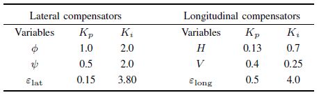
Furthermore,the longitudinal and lateral compensators were designed heuristically to eliminate the corresponding formation errors,and their parameters are listed in Table I.

To perform the computer simulations and evaluate the performance of the proposed formation control strategy,the nonlinear Aerosonde model was utilised with all the controller gains and parameters as shown previously.

B.Maintenance and Change of Multi-UAV Formation

To illustrate the performance of the maintenance and change during multi-UAV motion,several general assumptions and definitions are necessary to be given first:

1) The reference airspeed for all the vehicles with respect to the inertial reference frame is $26 $m/s,and the constraint on the airspeed is 15 $\sim$ 50 m/s. Also,the defined constraints on the pitch and roll angles are given as $\pm20 $deg and $\pm45 $deg,respectively.

2) All the UAVs were initially flying with the desired formation geometry as shown in Fig. 3 (a),where the formation communication topology is assumed to be bidirectional partial-mesh.

3) During the formation changes,the formation topology is maintained.

This topological structure of the multi-UAV formation is intuitively displayed in Fig. 3,where the diamond symbol labelled with number indicates the corresponding UAV,whereas UAV 2 acts as the reference vehicle,and ${T}_{i\leftrightarrow j}^{{F}}$,$i$,$j=1,2,3,4$, $i\neq j$ is to describe the reaction relationship between the UAVs. The double-headed arrow means that there exists the bidirectional reaction or interaction between the related UAVs. The altitude formation or the relative coordinates in the $Z_L$ axis are indicated by the neighboured annotations ($p_{Liz}$,$i=1,2,3,4$). Alternatively,the desired formation change process can be mathematically expressed by

\begin{align} &F_{d\_A}^{{p}} = \left[{\begin{array}{*{20}{c}} {-300}&{\ \ 300}&0\\ \ \ 0&\ \ 0&0\\{-150}&{-150}&0\\{-300}&{-300}&0 \end{array}} \right]\Rightarrow \nonumber\\[2mm] & F_{d\_B}^{{p}} = \left[{\begin{array}{*{20}{c}} {-150}&{\ \ 150}&0\\ \ \ 0&\ \ 0&0\\{-150}&{-300}&0\\{-300}&{-300}&{100} \end{array}} \right] \Rightarrow \nonumber\\[2mm] &F_{d\_C}^{{p}} = \left[{\begin{array}{*{20}{c}} {-150}&{\ \ 150}&{\ \ 100}\\ \ \ 0&\ \ 0&\ \ 0\\{-150}&{-300}&{-200}\\{-300}&{-150}&{-100} \end{array}} \right], \end{align}

(32)

where subscript "$d$" means the desired formation representation and superscript "${p}$" represents "position coordination" in the local-formation reference frame.

The designed scenario of the formation manoeuvre is illustrated as: 1) The group of UAVs is tasked to navigate in 3-D space with the constant reference heading angle $\psi_{\rm ref}$ $=$ $0$ rad; 2) Fig. 3 (a) shows the initial formation arrangement with the defined bidirectional partial-mesh formation topology; 3) All UAVs were flying steadily at an altitude $H$ $=$ $800$ m in the first stage. When $t=20$ s,the formation started to climb until their altitudes were equal to $900$ m; 4) Figs. 3 (b) and 3 (c) illustrate the 3-D formation changes at $t=80$ s and at $t=120$ s respectively.

For the whole simulation,the resulting 3-D motional trajectories of the UAV group are shown in Fig. 4. In order to facilitate the observation,the above 3-D flight trajectories are separately projected onto the horizontal and vertical planes. The resulting horizontal projection is shown in Fig. 5,and the vertical one is shown in Fig. 6 which represents the altitude dynamics. Furthermore,the achieved states and individual formation errors are displayed in Figs. 7 and 8, respectively.

Based on these figures,the following observations could be made:

1) As shown in Fig. 5,the planar formation geometry satisfies the desired formation shapes: the desired formations defined in Figs. 3 (b) and 3 (c) were obtained at about $t$ $=$ $120 $s and $t=210 $s,respectively. As shown in Fig. 6,the climbing flight and the altitude formation change were achieved with a satisfying performance.

2) The forward,lateral and altitude formations of the multi-UAVs were stable and followed the reference formation$'$s commands closely. This is an argument for supporting the result of the overall formation stability achieved in Section IV.

3) Variations in the velocities of the UAVs could be observed during the formation changes. This was necessary to rapidly achieve the new reference formation,for instance,UAV 1 needed to speed up to align itself with UAV 3 when $t$ $>$ $80 $s. Moreover,all the vehicles in the formation attained the reference speed of $26 $m/s once the new formation was achieved.

4) As depicted in Fig. 7,it is clear that the airspeed and attitude (pitch and roll) of each UAV remained within the specified constraints during the cooperative flight.

5) The individual formation errors are shown in Fig. 8. During the formation changes,the transient formation errors asymptotically converged to zero after the new formation was achieved. This means that all steady-state formation errors were effectively eliminated by the supplemented compensators.

VI. CONCLUDING REMARKS

In this paper, based on the given formation definition and the three types of formation stability definitions,the formation stability conjecture is first proposed,and the EDA strategy is then specified to support the decentralised formation controller design. Throughout the subsequent stability analysis, it is proven that with the support of the CMP system,the stabilisation of all the IASs is sufficient to guarantee the stability of the overall formation system. The designed decentralised controllers are used to reject the impact of the formation changes and maintain the stability of each IAS,and subsequently guarantee the overall formation stability. Simulation studies on Aerosonde UAVs have been carried out to verify the achieved formation stability result. Future work includes formation stability analysis under dynamic formation topologies, and application of the methodology presented in this paper to other multi-agent problem-solving.

ACKNOWLEDGEMENT

The authors would like to acknowledge the EPSRC under UK-China Science Bridge grant (EP/G042594/1) and Flight Test Center of Commercial Aircraft Corporation of China (COMAC).